Sliced Episode 11: Austin House Prices
Summary:
Background: In episode 11 of the 2021 series of Sliced, the competitors were given two hours in which to analyse a set of data on properties in the Austin area that were advertised on Zillow. The aim was to predict the house price, lumped into 5 categories.
My approach: I decided to use these data to illustrate the use of pipelines in mlr3. I identify commonly used words from the estate agents description of the property and use a pipeline to filter them and combine the selected keywords with the numerical descriptors of the property. I use a random forest model and measure performance using cross-validation. I tune both the number of filtered features and the hyperparameters of the random forest.
Result: Performance of the model was poor.
Conclusion: The analysis provided a good illustration of the use of pipelines in mlr3, but it did not result in a competitive model. I found myself falling into the trap that I often see in videos on the use of tidymodels; insufficient attention to the intermediate steps.
Introduction:
The data for episode 11 of Sliced 2021 can be downloaded from https://www.kaggle.com/c/sliced-s01e11-semifinals/. The competition organisers took the data from a US on-line estate agent called Zillow. The properties have been grouped into five price categories, which the competitors to predict. Evaluation was by multi-class logloss.
I use these data to demonstrate exploratory analysis with tables and the use of pipelines in mlr3. The tables are produced using a combination of dplyr, janitor::tabyl and kable.
I have written two methods posts entitled Introduction to mlr3 and Pipelines in mlr3. These posts give the background needed to understand the mlr3 components of this analysis.
Reading the data
It is my practice to read the data asis and to immediately save it in rds format within a directory called data/rData. For details of the way that I organise my analyses you should read my post called Sliced Methods Overview.
# --- setup: libraries & options ------------------------
library(tidyverse)

theme_set( theme_light())

# --- set home directory -------------------------------
home <- "C:/Projects/kaggle/sliced/s01-e11"

# --- read downloaded data -----------------------------
trainRawDF <- readRDS( file.path(home, "data/rData/train.rds") )

testRawDF <- readRDS( file.path(home, "data/rData/test.rds") )
Data Exploration:
As usual, I start by summarising the training data with the skimr package.
# --- summarise the training set -----------------------
skimr::skim(trainRawDF)
I have hidden the output, which in this case shows very little except that the training set has data on 10,000 properties and there is no missing data except for 1 house that lacks a textual description.
The response
The response is called priceRange. It is an ordered categorical variable with 5 levels $0-$250,000, $250,000-$350,000, $350,000-$450,000, $450,000-$650,000 and $650,000+.
The boundaries have been chosen to give a symmetrical distribution across the price range.
# --- count of response categories ----------------------
trainRawDF %>%
  count( priceRange)
## # A tibble: 5 x 2
## priceRange n
## <chr> <int>
## 1 0-250000 1249
## 2 250000-350000 2356
## 3 350000-450000 2301
## 4 450000-650000 2275
## 5 650000+ 1819Predictors
The location of the property is given in two ways, as a city and as a latitude and longitude. Here are the house prices by city.
library(knitr)
library(kableExtra)
# --- city ----------------------------------------------
trainRawDF %>%
  janitor::tabyl( priceRange, city) %>%
  janitor::adorn_totals("row") %>%
  kable(caption="House prices by City",
        col.names=c("Price",
                  substr(sort(unique(trainRawDF$city)),1,8))) %>%
kable_classic(full_width=FALSE)| Price | austin | del vall | driftwoo | dripping | manchaca | pflugerv | west lak |
|---|---|---|---|---|---|---|---|
| 0-250000 | 1189 | 54 | 0 | 0 | 0 | 6 | 0 |
| 250000-350000 | 2329 | 3 | 0 | 0 | 2 | 22 | 0 |
| 350000-450000 | 2299 | 0 | 0 | 0 | 1 | 1 | 0 |
| 450000-650000 | 2274 | 0 | 1 | 0 | 0 | 0 | 0 |
| 650000+ | 1807 | 0 | 7 | 3 | 0 | 0 | 2 |
| Total | 9898 | 57 | 8 | 3 | 3 | 29 | 2 |
Almost all of the houses are in Austin, so City will be of little use.
Austin does have a crescent shape with a wooded area that takes a bite out of the city. The expensive houses seem to be clustered in and around this bite. The cheaper housing is mostly in suburbs to the east of the city.
# --- location ----------------------------------------
trainRawDF %>%
  ggplot( aes(x=longitude, y=latitude, colour=priceRange)) +
  geom_point()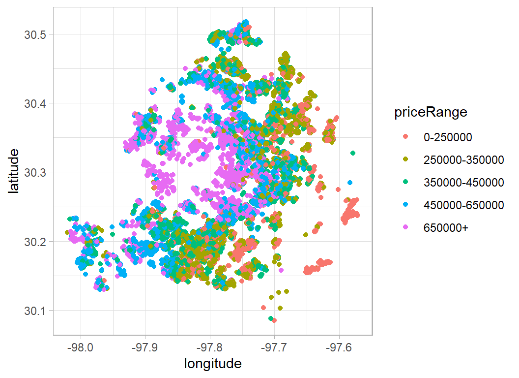
It looks as though the value depends on the distance from the centre, so it might be useful to plot polar coordinates.
# --- polar coordinates -------------------------------
mlat <- median(trainRawDF$latitude)
mlon <- median(trainRawDF$longitude)
trainRawDF %>%
  mutate( radius = sqrt( (latitude-mlat)^2 + (longitude-mlon)^2),
          angle = atan((latitude-mlat)/(longitude-mlon))) %>%
    ggplot( aes(x=radius, y=angle, colour=priceRange)) +
  geom_point()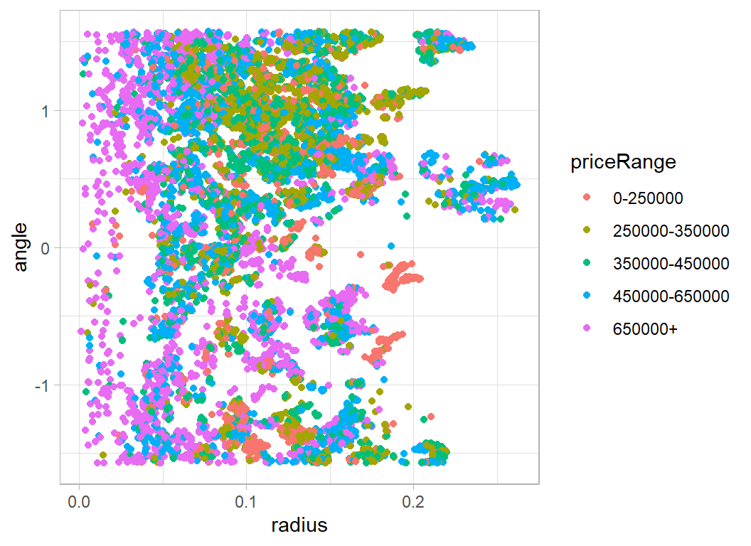
The other geographical predictors relate to local schooling. As you might expect, schooling is better if you are well-off. However, the worse schools seem to have fewer students for each teacher.
# --- table of measures of schooling -------------------
trainRawDF %>%
  group_by( priceRange) %>%
  summarise( n=n(),
             rating = mean(avgSchoolRating),
             ratio  = mean(MedianStudentsPerTeacher),
             .groups = "drop") %>%
  kable( digits=2,
         col.names = c("Price", "n", "school rating", "student ratio"),
         caption="House prices and local schools") %>%
kable_classic(full_width=FALSE)| Price | n | school rating | student ratio |
|---|---|---|---|
| 0-250000 | 1249 | 4.27 | 13.74 |
| 250000-350000 | 2356 | 4.80 | 14.10 |
| 350000-450000 | 2301 | 5.79 | 14.93 |
| 450000-650000 | 2275 | 6.68 | 15.62 |
| 650000+ | 1819 | 6.88 | 15.56 |
House type should be a useful predictor, but unfortunately most houses are described as single family dwellings.
# --- home type ----------------------------------------------
trainRawDF %>%
  janitor::tabyl( priceRange, homeType) %>%
  janitor::adorn_totals("row") %>%
  kable(caption="Price by type of home",
        col.names=c("Price",
                  substr(sort(unique(trainRawDF$homeType)),1,6))) %>%
kable_classic(full_width=FALSE)| Price | Apartm | Condo | Mobile | MultiF | Multip | Other | Reside | Single | Townho | Vacant |
|---|---|---|---|---|---|---|---|---|---|---|
| 0-250000 | 4 | 88 | 5 | 0 | 12 | 0 | 0 | 1108 | 32 | 0 |
| 250000-350000 | 3 | 73 | 1 | 0 | 15 | 0 | 7 | 2241 | 15 | 1 |
| 350000-450000 | 3 | 71 | 2 | 1 | 15 | 0 | 3 | 2178 | 27 | 1 |
| 450000-650000 | 5 | 65 | 1 | 1 | 13 | 1 | 12 | 2152 | 25 | 0 |
| 650000+ | 4 | 36 | 1 | 3 | 5 | 1 | 5 | 1748 | 14 | 2 |
| Total | 19 | 333 | 10 | 5 | 60 | 2 | 27 | 9427 | 113 | 4 |
Indicators of size include number of bathrooms. I am never sure with Americans whether bathroom is literal. Presumably some facilities are shared giving the multiples of 0.5.
# --- number of bathrooms -----------------------------------
trainRawDF %>%
  janitor::tabyl(  priceRange, numOfBathrooms) %>%
  kable(caption="Price and the number of bathrooms")%>%
  kable_classic(full_width=FALSE) %>%
add_header_above(c(" "=1,"Number of bathrooms"=15))|
Number of bathrooms
|
|||||||||||||||
|---|---|---|---|---|---|---|---|---|---|---|---|---|---|---|---|
| priceRange | 1 | 1.5 | 10 | 2 | 2.5 | 3 | 3.5 | 4 | 4.5 | 5 | 5.5 | 6 | 6.5 | 7 | 8 |
| 0-250000 | 147 | 2 | 0 | 733 | 24 | 320 | 1 | 18 | 0 | 1 | 0 | 2 | 0 | 0 | 1 |
| 250000-350000 | 172 | 2 | 0 | 1294 | 24 | 822 | 3 | 36 | 0 | 2 | 0 | 1 | 0 | 0 | 0 |
| 350000-450000 | 170 | 5 | 0 | 1096 | 19 | 864 | 4 | 138 | 1 | 4 | 0 | 0 | 0 | 0 | 0 |
| 450000-650000 | 95 | 4 | 0 | 670 | 14 | 950 | 14 | 479 | 1 | 38 | 0 | 5 | 0 | 2 | 3 |
| 650000+ | 38 | 1 | 2 | 237 | 5 | 602 | 7 | 599 | 1 | 208 | 1 | 80 | 1 | 33 | 4 |
As you would expect, the trend is, the greater the number of bedrooms, the higher the price. A similar pattern can be seen in the number of bedrooms.
# --- number of bedrooms -----------------------------------
trainRawDF %>%
  group_by( priceRange, numOfBedrooms) %>%
  summarise( n = n(), .groups="drop") %>%
  pivot_wider(values_from=n, names_from=numOfBedrooms, values_fill=0,
              names_sort=TRUE) %>%
kable(caption="Price and the number of bedrooms") %>%
  kable_classic(full_width=FALSE) %>%
add_header_above(c(" "=1,"Number of bedrooms"=9))|
Number of bedrooms
|
|||||||||
|---|---|---|---|---|---|---|---|---|---|
| priceRange | 1 | 2 | 3 | 4 | 5 | 6 | 7 | 8 | 10 |
| 0-250000 | 24 | 150 | 833 | 214 | 21 | 5 | 0 | 2 | 0 |
| 250000-350000 | 15 | 154 | 1564 | 577 | 40 | 5 | 0 | 1 | 0 |
| 350000-450000 | 17 | 160 | 1247 | 781 | 85 | 5 | 1 | 5 | 0 |
| 450000-650000 | 9 | 155 | 815 | 1013 | 265 | 12 | 2 | 3 | 1 |
| 650000+ | 4 | 69 | 460 | 868 | 376 | 35 | 4 | 3 | 0 |
These are US data, so one can never be certain, but it is likely that some of the larger numbers of garage spaces refer to shared parking for a group of properties.
# --- parking ---------------------------------------------
trainRawDF %>%
  group_by( priceRange, garageSpaces) %>%
  summarise( n = n(), .groups="drop") %>%
  pivot_wider(values_from=n, names_from=garageSpaces, values_fill=0,
              names_sort=TRUE) %>%
  kable(caption="Price and size of garage") %>%
  kable_classic(full_width=FALSE) %>%
add_header_above(c(" "=1,"Garage Spaces"=13))|
Garage Spaces
|
|||||||||||||
|---|---|---|---|---|---|---|---|---|---|---|---|---|---|
| priceRange | 0 | 1 | 2 | 3 | 4 | 5 | 6 | 7 | 8 | 9 | 10 | 12 | 22 |
| 0-250000 | 660 | 138 | 395 | 12 | 40 | 0 | 4 | 0 | 0 | 0 | 0 | 0 | 0 |
| 250000-350000 | 1183 | 170 | 888 | 27 | 71 | 4 | 9 | 0 | 1 | 0 | 2 | 1 | 0 |
| 350000-450000 | 1044 | 167 | 933 | 76 | 65 | 4 | 9 | 0 | 1 | 1 | 0 | 0 | 1 |
| 450000-650000 | 899 | 150 | 872 | 218 | 96 | 12 | 18 | 2 | 5 | 0 | 2 | 1 | 0 |
| 650000+ | 672 | 108 | 577 | 298 | 114 | 27 | 15 | 3 | 2 | 1 | 2 | 0 | 0 |
Number of patio & porch features also show the more you get the more expensive the property.
# --- Patio and Porch --------------------------------------
trainRawDF %>%
  group_by( priceRange, numOfPatioAndPorchFeatures) %>%
  summarise( n = n(), .groups="drop") %>%
  pivot_wider(values_from=n, names_from=numOfPatioAndPorchFeatures,
              values_fill=0, names_sort=TRUE) %>%
  kable(caption="Price and Patio/Porch features") %>%
  kable_classic(full_width=FALSE) %>%
add_header_above(c(" "=1,"Patio and Porch features"=9))|
Patio and Porch features
|
|||||||||
|---|---|---|---|---|---|---|---|---|---|
| priceRange | 0 | 1 | 2 | 3 | 4 | 5 | 6 | 7 | 8 |
| 0-250000 | 931 | 227 | 74 | 15 | 1 | 1 | 0 | 0 | 0 |
| 250000-350000 | 1525 | 470 | 274 | 68 | 18 | 1 | 0 | 0 | 0 |
| 350000-450000 | 1344 | 490 | 320 | 115 | 27 | 5 | 0 | 0 | 0 |
| 450000-650000 | 1250 | 466 | 375 | 146 | 31 | 5 | 1 | 1 | 0 |
| 650000+ | 1022 | 324 | 288 | 135 | 40 | 7 | 2 | 0 | 1 |
Having a spa is also associated with expensive properties.
# --- Spa -------------------------------------------------
trainRawDF %>%
  mutate( hasSpa = factor(hasSpa, levels=c(FALSE,TRUE),
                          labels=c("No","Yes"))) %>%
  group_by( priceRange, hasSpa) %>%
  summarise( n = n(), .groups="drop") %>%
  pivot_wider(values_from=n, names_from=hasSpa, values_fill=0,
              names_sort=TRUE) %>%
  kable(caption="Price and Spa") %>%
  kable_classic(full_width=FALSE) %>%
add_header_above(c(" "=1,"Spa"=2))|
Spa
|
||
|---|---|---|
| priceRange | No | Yes |
| 0-250000 | 1221 | 28 |
| 250000-350000 | 2243 | 113 |
| 350000-450000 | 2161 | 140 |
| 450000-650000 | 2057 | 218 |
| 650000+ | 1493 | 326 |
The lot size in square feet shows the expected trend of larger properties costing more, but with some oddities.
# --- area of the land -------------------------------------
trainRawDF %>%
  group_by( priceRange) %>%
  summarise( n       = n(),
             mean    = round(mean(lotSizeSqFt), 0),
             median  = round(median(lotSizeSqFt), 0),
             min     = min(lotSizeSqFt),
             max     = max(lotSizeSqFt),
             .groups = "drop") %>%
  kable(caption="Price and size of garage") %>%
kable_classic(full_width=FALSE)| priceRange | n | mean | median | min | max |
|---|---|---|---|---|---|
| 0-250000 | 1249 | 62553 | 6359 | 392 | 34154525 |
| 250000-350000 | 2356 | 8210 | 7143 | 113 | 435600 |
| 350000-450000 | 2301 | 11727 | 8058 | 100 | 2988216 |
| 450000-650000 | 2275 | 14660 | 9452 | 117 | 5880600 |
| 650000+ | 1819 | 27102 | 12197 | 217 | 8581320 |
Clearly there is a data problem. There are two properties with over 10 million square feet and both are cheap.
# --- log area by price ------------------------------------
trainRawDF %>%
   ggplot( aes(x=priceRange, y=log10(lotSizeSqFt))) +
   geom_boxplot()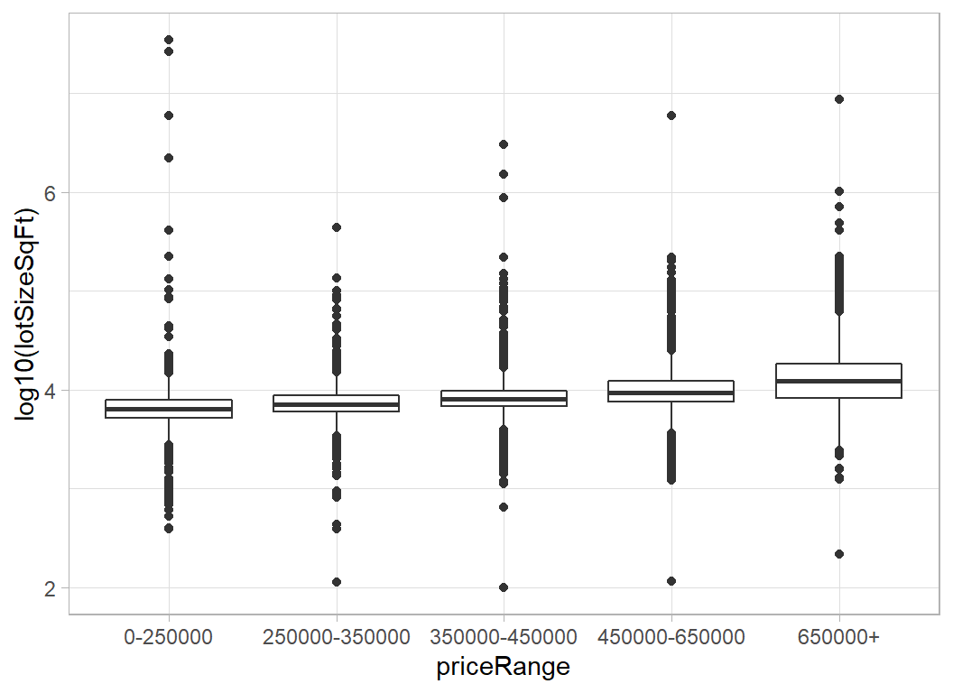
Let look at the descriptions of the largest properties.
trainRawDF %>%
  filter( lotSizeSqFt > 5000000) %>%
  pull( description)
## [1] "Leased for $1695 though 7/31/2020 - Unique gated community, quiet, and one of the most sought after locations in West Campus, 2 (TWO) parking spaces, High ceilings, split level 2 bedroom (one is a loft), one bath with marble & custom laminate floors which were recently replaced. Private deck-close to UT & downtown- Leased for $1695 though 7/31/2020"
## [2] "**Subject to City of Austin SMART Housing and Mueller Foundation Affordable Home Program requirements. (80% MFI). BUYER MUST HAVE PRE-QUALIFICATION** See Process/COVID docs for application process. Walk to Thinkery, Drafthouse, HEB, hike & bike trails, playgrounds/community pools. Great Community to Live, Work, and Play! This isa resale-restricted home and must be sold to an income-qualified buyers. See Docs/Agent for details.**"
## [3] "Rare 2 story home with 5 bed, 4.5 bath, dedicated office, game room AND theater room. One of the most desired features of this home is the 2 spacious master suites downstairs with 2 full + 1/2 bathrooms. This home shows like a model home with features ranging from stunning hardwoods, high-end finishes, tankless water heater, vaulted ceilings, recessed lighting, built-in speakers, stunning cast stone gas fireplace, granite countertops throughout the home to an outdoor living area with a built-in kitchen and BBQ grill. Luxury master suite has an oversized frameless shower enclosure and drop-in garden tub. The game room offers an additional living space. The theater room provides the key to a relaxing night in. Excellent Round Rock ISD schools and neighborhood amenities.\r\n\r\nThis home is professionally listed by Eric Peterson at Kopa Real Estate. Call 512-791-7473 or email eric@koparealestate.com for more information."
## [4] "201 Charismatic Pl, Austin, TX 78737 is a single family home that contains 4,459 sq ft and was built in 2015. It contains 5 bedrooms and 6 bathrooms. \r\n \r\n"
## [5] "Newly remodeled 3-2 conveniently located in Brushy Creek. This is an open floor plan that feels much larger than the stated size. New features include fresh paint, tile, carpet, fixtures, new furnace, new exterior doors, blinds, etc. New 30 year roof installed this year. One car garage with opener. Has two large master bedrooms and one smaller. Ceiling fans throughout. Gas heat and cooking. Large back yard. Planter beds in the front are ready for your personal touch.This is a MUST SEE nice home with great neighbors. Ready to move in and enjoy!\r\n\r\nNeighborhood Description\r\n\r\nGreat family oriented neighborhood in walking distance of exemplary Brushy Creek Elementary school. Walk to parks and trails. Convenient central location. Must see this one!"Five million square feet equates to over 100 acres. I find it hard to believe that affordable housing is on such a grand scale [2].
The very small lots also seem unlikely. 100 square feet is the size of a box room.
Removing the extremes provides a more believable distribution.
mSize <- median(trainRawDF$lotSizeSqFt)

trainRawDF %>%
  mutate( lotSizeSqFt = ifelse(lotSizeSqFt > 1000000 |
                               lotSizeSqFt < 300, mSize,
                               lotSizeSqFt) ) %>%
  group_by( priceRange) %>%
  summarise( n       = n(),
             mean    = round(mean(lotSizeSqFt), 0),
             median  = round(median(lotSizeSqFt), 0),
             min     = min(lotSizeSqFt),
             max     = max(lotSizeSqFt),
             .groups = "drop") %>%
  kable(caption="Price and size of garage") %>%
kable_classic(full_width=FALSE)| priceRange | n | mean | median | min | max |
|---|---|---|---|---|---|
| 0-250000 | 1249 | 7751 | 6359 | 392 | 411206.4 |
| 250000-350000 | 2356 | 8213 | 7143 | 392 | 435600.0 |
| 350000-450000 | 2301 | 9783 | 8058 | 644 | 871200.0 |
| 450000-650000 | 2275 | 12082 | 9452 | 1219 | 219542.4 |
| 650000+ | 1819 | 21846 | 12197 | 1258 | 702622.8 |
The other thing that we know is the year when the house was built; this does not look particularly predictive of price.
# --- year built -----------------------------------
trainRawDF %>%
   ggplot( aes(x=priceRange, y=yearBuilt)) +
   geom_boxplot()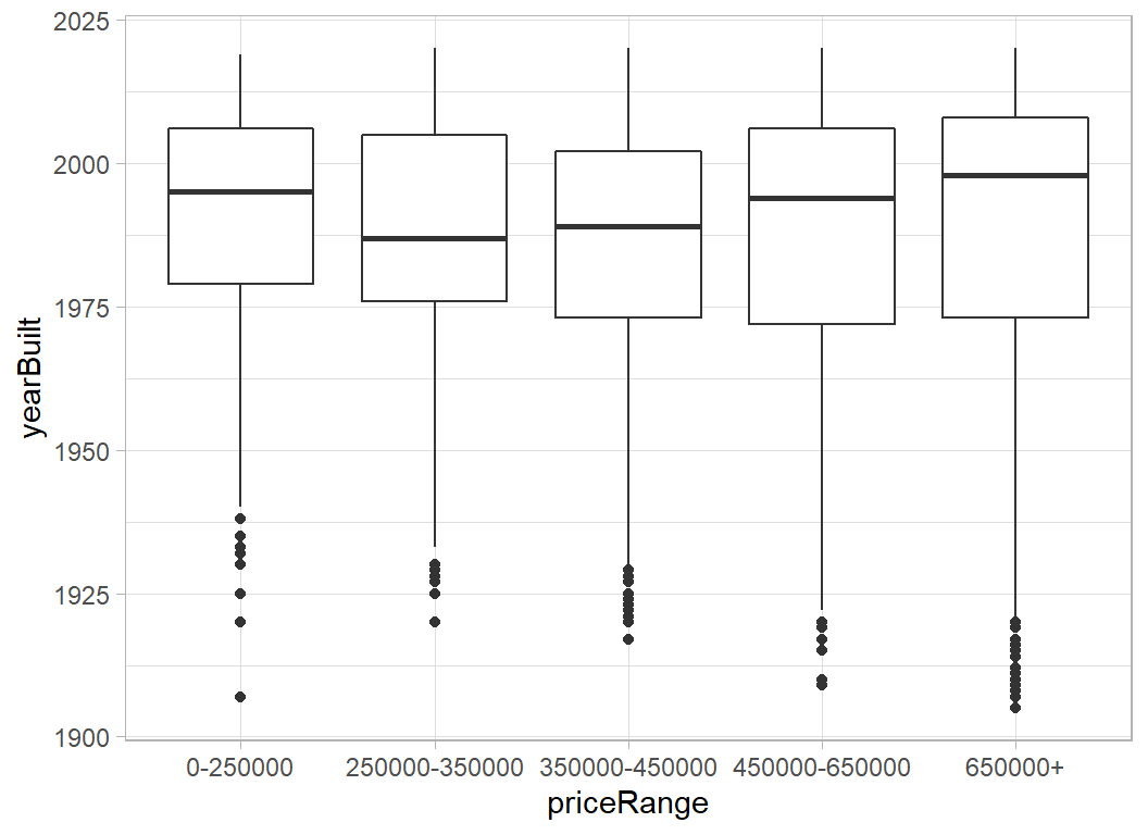
House Descriptions
In previous posts analysing other episodes of Slided, I have used my own functions for handling text, but here the text is longer and unstructured so it is worth using a package. tidytext would do the job, but I will use quanteda, because quanteda is integrated into mlr3 and it is a good package in its own right.
Here is a function built with quanteda that extracts words that occur at least some specified minimum number of times.
stopwordsare words such as “the”, "“a”, “and”, “on”, etc
stemsare the roots of words, so “bedroom” and “bedrooms” are united as “bedroom”, “great” and “greatly” are combined and so on.
# --- function to extract common words -------------------------
# arguments
#   text ... vector of character strings (the text)
#   minCount ... words must occur at least this many times
#   minLength ... minimum length of an eligible word
#   prefix ... prefix for a variable that counts the number of
#              occurrences in each string
# returns
#   tibble containing the indicators.
#
# uses the quanteda package
#
text_indicators <- function(text, minCount, minLength,
                            prefix="X") {
  library(quanteda)

  # --- extract the words -------------------------
  tokens(text, remove_punct=TRUE,
               remove_numbers=TRUE,
               remove_symbols=TRUE)  %>%
  # --- remove English stopwords ------------------
     tokens_remove(stopwords("en")) %>%
  # --- find words stems --------------------------
     tokens_wordstem() %>%
  # --- create indicators -------------------------
     dfm() %>%
     as.matrix() %>%
     as_tibble() -> mDF
  # --- remove if too rare  -----------------------
  mDF[, names(mDF)[apply(mDF, 2, sum) >= minCount]] -> mDF
  # --- remove if too ahort -----------------------
  mDF[, names(mDF)[str_length(names(mDF)) >= minLength]] -> mDF
  # --- create variable names ---------------------
  keywords <- names(mDF)
  names(mDF) <- paste(prefix, ".", names(mDF), sep="")
  return( mDF)
}
I will use the function to extract common words from the property description and construct indicator variables to show the number of times that the words occur in each description.
# --- DF of indicators for commonly occurring words --------------------
trainRawDF %>%
  mutate( description = ifelse( is.na(description), "", description)) %>%
  { text_indicators(.[["description"]],
                    200, 3,
                    prefix = "desc")} %>%
  print() -> indicatorDF
## # A tibble: 10,000 x 394
## desc.best desc.agent desc.rare desc.view desc.lot desc.see desc.home desc.sit
## <dbl> <dbl> <dbl> <dbl> <dbl> <dbl> <dbl> <dbl>
## 1 1 2 1 1 1 1 2 1
## 2 0 0 0 0 0 0 1 0
## 3 0 0 0 0 0 0 1 0
## 4 0 0 0 0 1 0 2 0
## 5 0 0 0 0 0 0 1 0
## 6 0 0 0 0 0 0 1 0
## 7 0 0 0 1 1 1 3 0
## 8 0 0 0 0 0 0 0 0
## 9 0 1 0 0 1 0 3 0
## 10 0 0 0 0 0 0 0 0
## # ... with 9,990 more rows, and 386 more variables: `desc.cul-de-sac` <dbl>,
## # desc.back <dbl>, desc.stun <dbl>, desc.remodel <dbl>, desc.kitchen <dbl>,
## # desc.bathroom <dbl>, desc.master <dbl>, desc.suit <dbl>, desc.privat <dbl>,
## # desc.bath <dbl>, desc.huge <dbl>, desc.bedroom <dbl>, `desc.walk-in` <dbl>,
## # desc.closet <dbl>, desc.deck <dbl>, desc.pool <dbl>, desc.park <dbl>,
## # desc.tenni <dbl>, desc.court <dbl>, desc.high <dbl>, desc.well <dbl>,
## # desc.love <dbl>, desc.featur <dbl>, desc.live <dbl>, desc.area <dbl>,
## # desc.offic <dbl>, desc.car <dbl>, desc.garag <dbl>, desc.austin <dbl>,
## # desc.singl <dbl>, desc.famili <dbl>, desc.contain <dbl>, desc.built <dbl>,
## # desc.beauti <dbl>, desc.larg <dbl>, desc.tree <dbl>, desc.light <dbl>,
## # desc.spacious <dbl>, desc.dine <dbl>, desc.room <dbl>, desc.open <dbl>,
## # desc.floor <dbl>, desc.plan <dbl>, desc.layout <dbl>, desc.yard <dbl>,
## # desc.newli <dbl>, desc.patio <dbl>, `desc.built-in` <dbl>, desc.shed <dbl>,
## # desc.new <dbl>, desc.lamin <dbl>, desc.tile <dbl>, desc.throughout <dbl>,
## # desc.renov <dbl>, desc.upgrade <dbl>, desc.stainless <dbl>,
## # desc.applianc <dbl>, desc.washer <dbl>, desc.dryer <dbl>,
## # desc.laundri <dbl>, desc.util <dbl>, desc.recess <dbl>, desc.ceil <dbl>,
## # desc.fan <dbl>, desc.neighborhood <dbl>, desc.locat <dbl>,
## # desc.north <dbl>, desc.citi <dbl>, desc.south <dbl>, desc.first <dbl>,
## # desc.east <dbl>, desc.hill <dbl>, desc.design <dbl>, desc.oak <dbl>,
## # desc.wonder <dbl>, desc.bright <dbl>, desc.concept <dbl>, desc.vault <dbl>,
## # desc.formal <dbl>, desc.gorgeous <dbl>, desc.custom <dbl>, desc.wood <dbl>,
## # desc.cabinetri <dbl>, desc.quartz <dbl>, desc.countertop <dbl>,
## # desc.doubl <dbl>, desc.pantri <dbl>, desc.breakfast <dbl>,
## # desc.hardwood <dbl>, desc.fantast <dbl>, desc.exterior <dbl>,
## # desc.side <dbl>, desc.window <dbl>, desc.system <dbl>, desc.landscap <dbl>,
## # desc.contemporari <dbl>, desc.corner <dbl>, desc.entertain <dbl>,
## # desc.floorplan <dbl>, desc.attach <dbl>, ...It would be interesting to know which words are associated with price. I will use a kruskal-wallis nonparameteric test to assess the association
# --- kruskal-wallis test of counts vs priceRange ------------------
trainRawDF %>%
  select( priceRange) %>%
  bind_cols(indicatorDF) %>%
  pivot_longer(starts_with("d"), names_to="var", values_to="count") %>%
  group_by( var) %>%
  summarise( p = kruskal.test(count, priceRange)$p.value, .groups="drop") %>%
  filter( p < 0.05) %>%
  arrange( p ) %>%
  print()             -> keyVarDF
## # A tibble: 293 x 2
## var p
## <chr> <dbl>
## 1 desc.view 1.47e-108
## 2 desc.outdoor 2.32e- 94
## 3 desc.hill 4.89e- 90
## 4 desc.countri 1.84e- 88
## 5 desc.spa 4.87e- 84
## 6 desc.barton 7.02e- 74
## 7 desc.pool 3.10e- 65
## 8 desc.custom 9.91e- 58
## 9 desc.gourmet 5.02e- 56
## 10 desc.media 2.01e- 55
## # ... with 283 more rowsindicatorDF contains 394 words that occur at least 200 times in the property descriptions and keyvarDF contains 293 words that show a nominally significant relationship with priceRange.
Pre-processing
I want to continue the theme from episode 10 and illustrate some more aspects of mlr3. In particular, I want to run the pre-process using mlr3 rather than writing my own code as I usually do. My eventual plan for the analysis is to use a random forest model.
The data cleaning will consist of
- convert
priceRangefrom a character to a factor
- if
descriptionis missing replace it with an empty string
- convert the logical
hasSpato a numerical 0/1
- encode the factors
cityandhometypeas indicators (dummy variables)
- encode the keywords from the
description
Having cleaned the data, I plan to introduce a filter whereby I select the best keywords for inclusion in the predictive model. I will treat the number of keywords, n, as a hyperparameter and tune the model to find the best value of n.
Data cleaning
First I perform those pre-processing steps that I judge will not change materially whether I run them on the full training data or a subset of it, i.e. I do not anticipate a problem of data leakage.
library(tidyverse)

# --- set home directory -------------------------------
home <- "C:/Projects/kaggle/sliced/s01-e11"

# --- read downloaded data -----------------------------
trainRawDF <- readRDS( file.path(home, "data/rData/train.rds") ) %>%
                mutate( priceRange = factor(priceRange))

testRawDF <- readRDS( file.path(home, "data/rData/test.rds") )

# --- function to clean a data set ---------------------
pre_process <- function(thisDF) {
   # --- median lat and long ---------------------------
   mlat  <- median(trainRawDF$latitude)
   mlon  <- median(trainRawDF$longitude)
   # --- median lot size -------------------------------
   mSize <- median(trainRawDF$lotSizeSqFt)

   thisDF %>%
      # --- city = Austin or Other ---------------------
      mutate( city = factor(city=="austin", levels=c(TRUE, FALSE),
                           labels=c("Austin", "Other")),
      # --- combine multiple categories ----------------
              homeType  = factor(
                          ifelse( homeType == "MultiFamily" |
                                  homeType == "Multiple Occupancy",
                                  "Multiple", homeType)),
      # --- remove extreme lot sizes -------------------
              lotSizeSqFt = ifelse(lotSizeSqFt > 1000000 |
                               lotSizeSqFt < 300, mSize,
                               lotSizeSqFt),
      # --- missing description converted to "" --------
              description = ifelse( is.na(description), "",
                                    description),
      # --- hasSpa to numeric (0/1) --------------------
              hasSpa = as.numeric(hasSpa),
      # --- polar coordinates --------------------------
              radius = sqrt( (latitude-mlat)^2 + (longitude-mlon)^2),
              angle = atan((latitude-mlat)/(longitude-mlon)))  %>%
  return()
}

trainDF <- pre_process(trainRawDF)

# --- combine indicators with clean training data -----
trainDF <- bind_cols( trainDF %>%
                      select( -description, -uid),
                      indicatorDF)

# --- remove the hyphens from the column names ------------
names(trainDF) <- str_replace_all(names(trainDF), "-", "_")

trainDF
## # A tibble: 10,000 x 410
## city homeType latitude longitude garageSpaces hasSpa yearBuilt
## <fct> <fct> <dbl> <dbl> <dbl> <dbl> <dbl>
## 1 Aust~ Single ~ 30.4 -97.8 0 0 1988
## 2 Aust~ Single ~ 30.2 -97.9 0 0 1997
## 3 Aust~ Single ~ 30.2 -97.7 0 0 1952
## 4 Aust~ Single ~ 30.2 -97.8 4 0 1976
## 5 Aust~ Single ~ 30.3 -97.8 2 0 1984
## 6 Aust~ Single ~ 30.2 -97.8 0 0 1964
## 7 Aust~ Single ~ 30.3 -97.9 0 0 2015
## 8 Aust~ Multiple 30.3 -97.7 1 0 1967
## 9 Aust~ Single ~ 30.2 -97.8 2 0 1983
## 10 Aust~ Single ~ 30.4 -97.7 0 0 1972
## # ... with 9,990 more rows, and 403 more variables:
## # numOfPatioAndPorchFeatures <dbl>, lotSizeSqFt <dbl>, avgSchoolRating <dbl>,
## # MedianStudentsPerTeacher <dbl>, numOfBathrooms <dbl>, numOfBedrooms <dbl>,
## # priceRange <fct>, radius <dbl>, angle <dbl>, desc.best <dbl>,
## # desc.agent <dbl>, desc.rare <dbl>, desc.view <dbl>, desc.lot <dbl>,
## # desc.see <dbl>, desc.home <dbl>, desc.sit <dbl>, desc.cul_de_sac <dbl>,
## # desc.back <dbl>, desc.stun <dbl>, desc.remodel <dbl>, desc.kitchen <dbl>,
## # desc.bathroom <dbl>, desc.master <dbl>, desc.suit <dbl>, desc.privat <dbl>,
## # desc.bath <dbl>, desc.huge <dbl>, desc.bedroom <dbl>, desc.walk_in <dbl>,
## # desc.closet <dbl>, desc.deck <dbl>, desc.pool <dbl>, desc.park <dbl>,
## # desc.tenni <dbl>, desc.court <dbl>, desc.high <dbl>, desc.well <dbl>,
## # desc.love <dbl>, desc.featur <dbl>, desc.live <dbl>, desc.area <dbl>,
## # desc.offic <dbl>, desc.car <dbl>, desc.garag <dbl>, desc.austin <dbl>,
## # desc.singl <dbl>, desc.famili <dbl>, desc.contain <dbl>, desc.built <dbl>,
## # desc.beauti <dbl>, desc.larg <dbl>, desc.tree <dbl>, desc.light <dbl>,
## # desc.spacious <dbl>, desc.dine <dbl>, desc.room <dbl>, desc.open <dbl>,
## # desc.floor <dbl>, desc.plan <dbl>, desc.layout <dbl>, desc.yard <dbl>,
## # desc.newli <dbl>, desc.patio <dbl>, desc.built_in <dbl>, desc.shed <dbl>,
## # desc.new <dbl>, desc.lamin <dbl>, desc.tile <dbl>, desc.throughout <dbl>,
## # desc.renov <dbl>, desc.upgrade <dbl>, desc.stainless <dbl>,
## # desc.applianc <dbl>, desc.washer <dbl>, desc.dryer <dbl>,
## # desc.laundri <dbl>, desc.util <dbl>, desc.recess <dbl>, desc.ceil <dbl>,
## # desc.fan <dbl>, desc.neighborhood <dbl>, desc.locat <dbl>,
## # desc.north <dbl>, desc.citi <dbl>, desc.south <dbl>, desc.first <dbl>,
## # desc.east <dbl>, desc.hill <dbl>, desc.design <dbl>, desc.oak <dbl>,
## # desc.wonder <dbl>, desc.bright <dbl>, desc.concept <dbl>, desc.vault <dbl>,
## # desc.formal <dbl>, desc.gorgeous <dbl>, desc.custom <dbl>, desc.wood <dbl>,
## # desc.cabinetri <dbl>, ...Modelling
Task definition
I will now switch to mlr3. The first job is to define the task, which in this case is to classify priceRange using trainDF.
library(mlr3verse)

myTask <- TaskClassif$new(
               id      = "Austin housing",
               backend = trainDF,
               target  = "priceRange")
PipeOps
As I explain in my post "Methods: Pipelines in mlr3*. I do not like the names that mlr3 gives to its helper functions; the names are to short for my taste and I keep forgetting what they do. So I have renamed them. You, of course, are free to use the original names.
# === NEW NAMES FOR THE HELPER FUNCTIONS =======================

# --- po() creates a pipe operator -----------------------------
pipeOp <- function(...) po(...)

# --- lrn() creates an instance of learner ---------------------
setModel <- function(...) lrn(...)

# --- rsmp() creates a resampler -------------------------------
setSampler <- function(...) rsmp(...)

# --- msr() creates a measure ----------------------------------
setMeasure <- function(...) msr(...)

# --- flt() creates a filter ----------------------------------
setFilter <- function(...) flt(...)
I want to convert the two factors (city and homeType) into dummy variables. I could have done this in dplyr, but it is a good example to start with, when explaining pre-processing in mlr3.
I define two encoding PipeOps using mlr3s helper (sugar) function po(), renamed pipeOp. treatment encoding omits the first level of the factor, so I get a single numeric variable that is 0 for Austin and 1 for Other. homeType has 5 levels and I opt for one-hot encoding; this give 5 indicators one for each level.
The two PipeOps are given the names encCityOp and encHomeTypeOp.
# --- encode City ----------------------------------
encCityOp = pipeOp("encode",
                   id             = "encCity",
                   method         = "treatment",
                   affect_columns = selector_name("city"))

# --- encode HouseType -----------------------------
encHomeTypeOp = pipeOp("encode",
                       id             = "encHome",
                       method         = "one-hot",
                       affect_columns = selector_name("homeType"))
Next I want to run a filter on the features, 394 is simply too many for a random forest and I am sure that most of them would not contribute. mlr3 offers a wide range of filters. They are stored in a dictionary and we can list them
library("mlr3filters")

mlr_filters
## <DictionaryFilter> with 19 stored values
## Keys: anova, auc, carscore, cmim, correlation, disr, find_correlation,
## importance, information_gain, jmi, jmim, kruskal_test, mim, mrmr,
## njmim, performance, permutation, relief, varianceI stick with the kruskal-wallis test that I used earlier and create a filter using the helper function flt() renamed to setFilter()
kwFilter <- setFilter("kruskal_test") I need to put this filter into a PipeOp and then add it to the pipeline. To start with I will perform the K-W test and then pick the top 20 features.
Individual PipeOps can operate on multiple tasks, but a pipeline always starts with a single set of data, so not need for a list() when I train a pipeline.
kwFilterOp <- pipeOp("filter",
                     filter       = kwFilter,
                     filter.nfeat = 20)
Let’s see which features would get selected.
encCityOp %>>%
  encHomeTypeOp %>>%
  kwFilterOp     ->   myPipeline

myPipeline$train( myTask)
## $kruskal_test.output
## <TaskClassif:Austin housing> (10000 x 21)
## * Target: priceRange
## * Properties: multiclass
## * Features (20):
## - dbl (20): MedianStudentsPerTeacher, angle, avgSchoolRating,
## desc.barton, desc.countri, desc.custom, desc.gourmet, desc.hill,
## desc.media, desc.outdoor, desc.pool, desc.spa, desc.view,
## garageSpaces, hasSpa, longitude, lotSizeSqFt, numOfBathrooms,
## numOfBedrooms, radiusLatitude does not make the top 20 features, which I find surprising. The likely reason is that radius was preferred.
In the spirit of the demonstration of pieplines, I’ll suppose that I want to force latitude into the model. In fact, I go further and pick out all of the continuous variables and force them into the feature set and I’ll run the filter only on the indicator variables.
Here are the names of the features that I will select from
# --- description indicators ---------------------------------
trainDF %>%
  select( starts_with("desc")) %>%
  names() %>%
  print() -> descVars
## [1] "desc.best" "desc.agent" "desc.rare"
## [4] "desc.view" "desc.lot" "desc.see"
## [7] "desc.home" "desc.sit" "desc.cul_de_sac"
## [10] "desc.back" "desc.stun" "desc.remodel"
## [13] "desc.kitchen" "desc.bathroom" "desc.master"
## [16] "desc.suit" "desc.privat" "desc.bath"
## [19] "desc.huge" "desc.bedroom" "desc.walk_in"
## [22] "desc.closet" "desc.deck" "desc.pool"
## [25] "desc.park" "desc.tenni" "desc.court"
## [28] "desc.high" "desc.well" "desc.love"
## [31] "desc.featur" "desc.live" "desc.area"
## [34] "desc.offic" "desc.car" "desc.garag"
## [37] "desc.austin" "desc.singl" "desc.famili"
## [40] "desc.contain" "desc.built" "desc.beauti"
## [43] "desc.larg" "desc.tree" "desc.light"
## [46] "desc.spacious" "desc.dine" "desc.room"
## [49] "desc.open" "desc.floor" "desc.plan"
## [52] "desc.layout" "desc.yard" "desc.newli"
## [55] "desc.patio" "desc.built_in" "desc.shed"
## [58] "desc.new" "desc.lamin" "desc.tile"
## [61] "desc.throughout" "desc.renov" "desc.upgrade"
## [64] "desc.stainless" "desc.applianc" "desc.washer"
## [67] "desc.dryer" "desc.laundri" "desc.util"
## [70] "desc.recess" "desc.ceil" "desc.fan"
## [73] "desc.neighborhood" "desc.locat" "desc.north"
## [76] "desc.citi" "desc.south" "desc.first"
## [79] "desc.east" "desc.hill" "desc.design"
## [82] "desc.oak" "desc.wonder" "desc.bright"
## [85] "desc.concept" "desc.vault" "desc.formal"
## [88] "desc.gorgeous" "desc.custom" "desc.wood"
## [91] "desc.cabinetri" "desc.quartz" "desc.countertop"
## [94] "desc.doubl" "desc.pantri" "desc.breakfast"
## [97] "desc.hardwood" "desc.fantast" "desc.exterior"
## [100] "desc.side" "desc.window" "desc.system"
## [103] "desc.landscap" "desc.contemporari" "desc.corner"
## [106] "desc.entertain" "desc.floorplan" "desc.attach"
## [109] "desc.door" "desc.wall" "desc.outdoor"
## [112] "desc.spa" "desc.invit" "desc.countri"
## [115] "desc.much" "desc.use" "desc.full"
## [118] "desc.multipl" "desc.like" "desc.upgrad"
## [121] "desc.must" "desc.minut" "desc.away"
## [124] "desc.great" "desc.restaur" "desc.shop"
## [127] "desc.easi" "desc.access" "desc.unit"
## [130] "desc.bed" "desc.amaz" "desc.texa"
## [133] "desc.boast" "desc.central" "desc.2nd"
## [136] "desc.along" "desc.loft" "desc.space"
## [139] "desc.mopac" "desc.pleas" "desc.call"
## [142] "desc.show" "desc.owner" "desc.work"
## [145] "desc.properti" "desc.walk" "desc.distanc"
## [148] "desc.creek" "desc.cozi" "desc.fireplac"
## [151] "desc.make" "desc.perfect" "desc.granit"
## [154] "desc.steel" "desc.cabinet" "desc.size"
## [157] "desc.updat" "desc.vaniti" "desc.4th"
## [160] "desc.play" "desc.complet" "desc.backyard"
## [163] "desc.extend" "desc.last" "desc.long"
## [166] "desc.readi" "desc.front" "desc.allow"
## [169] "desc.separ" "desc.flow" "desc.garden"
## [172] "desc.domain" "desc.hous" "desc.greenbelt"
## [175] "desc.trail" "desc.solar" "desc.panel"
## [178] "desc.white" "desc.carpet" "desc.look"
## [181] "desc.outsid" "desc.energi" "desc.effici"
## [184] "desc.offer" "desc.price" "desc.just"
## [187] "desc.downtown" "desc.near" "desc.ton"
## [190] "desc.plenti" "desc.guest" "desc.cover"
## [193] "desc.porch" "desc.miss" "desc.opportun"
## [196] "desc.situat" "desc.enjoy" "desc.natur"
## [199] "desc.includ" "desc.roof" "desc.hvac"
## [202] "desc.water" "desc.heater" "desc.paint"
## [205] "desc.move_in" "desc.one" "desc.list"
## [208] "desc.avail" "desc.three" "desc.main"
## [211] "desc.finish" "desc.interior" "desc.ideal"
## [214] "desc.style" "desc.gourmet" "desc.neighbor"
## [217] "desc.game" "desc.bar" "desc.everi"
## [220] "desc.heat" "desc.buyer" "desc.desir"
## [223] "desc.zone" "desc.close" "desc.center"
## [226] "desc.market" "desc.amaze" "desc.quiet"
## [229] "desc.everyth" "desc.take" "desc.lead"
## [232] "desc.stori" "desc.brand" "desc.min"
## [235] "desc.sprinkler" "desc.ranch" "desc.street"
## [238] "desc.place" "desc.year" "desc.touch"
## [241] "desc.french" "desc.convey" "desc.hot"
## [244] "desc.tub" "desc.coffe" "desc.charm"
## [247] "desc.heart" "desc.plumb" "desc.electr"
## [250] "desc.mani" "desc.modern" "desc.backsplash"
## [253] "desc.old" "desc.gem" "desc.maintain"
## [256] "desc.sought" "desc.top" "desc.school"
## [259] "desc.amen" "desc.surround" "desc.replac"
## [262] "desc.fulli" "desc.storag" "desc.brick"
## [265] "desc.counter" "desc.sink" "desc.conveni"
## [268] "desc.crown" "desc.mold" "desc.dual"
## [271] "desc.level" "desc.set" "desc.fresh"
## [274] "desc.elementari" "desc.shade" "desc.condo"
## [277] "desc.communiti" "desc.nestl" "desc.fabul"
## [280] "desc.fenc" "desc.within" "desc.block"
## [283] "desc.quick" "desc.barton" "desc.acr"
## [286] "desc.creat" "desc.feel" "desc.abund"
## [289] "desc.upstair" "desc.island" "desc.matur"
## [292] "desc.less" "desc.mile" "desc.concret"
## [295] "desc.second" "desc.two" "desc.bike"
## [298] "desc.lake" "desc.balconi" "desc.uniqu"
## [301] "desc.squar" "desc.build" "desc.need"
## [304] "desc.addit" "desc.want" "desc.privaci"
## [307] "desc.downstair" "desc.major" "desc.apple"
## [310] "desc.round" "desc.rock" "desc.isd"
## [313] "desc.short" "desc.golf" "desc.insid"
## [316] "desc.soar" "desc.dream" "desc.luxuri"
## [319] "desc.nearbi" "desc.studi" "desc.welcom"
## [322] "desc.stone" "desc.relax" "desc.shower"
## [325] "desc.extra" "desc.friend" "desc.grill"
## [328] "desc.fridg" "desc.step" "desc.gas"
## [331] "desc.rang" "desc.plus" "desc.low"
## [334] "desc.chef" "desc.instal" "desc.come"
## [337] "desc.appeal" "desc.update" "desc.glass"
## [340] "desc.entri" "desc.fixtur" "desc.nice"
## [343] "desc.hike" "desc.retreat" "desc.airport"
## [346] "desc.origin" "desc.dishwash" "desc.hoa"
## [349] "desc.expans" "desc.overs" "desc.provid"
## [352] "desc.oasi" "desc.oven" "desc.big"
## [355] "desc.hard" "desc.commun" "desc.media"
## [358] "desc.recent" "desc.overlook" "desc.can"
## [361] "desc.clean" "desc.line" "desc.detail"
## [364] "desc.also" "desc.marbl" "desc.drive"
## [367] "desc.construct" "desc.shelv" "desc.bonus"
## [370] "desc.district" "desc.middl" "desc.screen"
## [373] "desc.popular" "desc.peac" "desc.playground"
## [376] "desc.ampl" "desc.end" "desc.gate"
## [379] "desc.lush" "desc.secondari" "desc.move"
## [382] "desc.green" "desc.steiner" "desc.around"
## [385] "desc.mueller" "desc.flex" "desc.shutter"
## [388] "desc.find" "desc.spring" "desc.meadow"
## [391] "desc.half" "desc.refriger" "desc.rate"
## [394] "desc.detach"Here is my plan. I’ll duplicate the data, from one copy I’ll extract the continuous features and scale them (using median and MAD), from the other copy of the data I’ll extract the description features and then I’ll run the filter on them selecting the top 20. Finally, I’ll combine the two sets of selected features.
Several of the PipeOps are defined in place when I create the pipeline.
# --- PipeOp to select non-description variables -------------------
selectOrigOp <- pipeOp("select",
                       id       = "selectOriginal",
                       selector = selector_invert(selector_name(descVars)))

# --- PipeOp to select description variables --------------
selectDescOp <- pipeOp("select",
                       id       = "selectDescOp",
                       selector = selector_name(descVars))

# --- Create a branched pipeline ---------------------------------
encCityOp %>>%
encHomeTypeOp %>>%
pipeOp("copy", outnum = 2) %>>%
gunion(list(
  # --- branch 1 ----
  selectOrigOp %>>%
    pipeOp("scale", robust=TRUE),
  # --- branch 2 ----
  selectDescOp %>>%
    kwFilterOp )
  ) %>>%
pipeOp("featureunion") -> myPipeline

# --- Plot the pipeline ------------------------------------------
plot(myPipeline)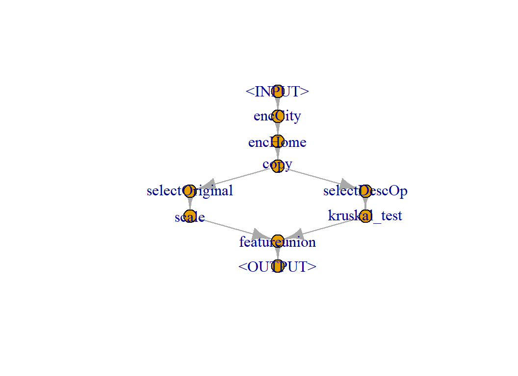
# --- train the pipeline -----------------------------------------
myPipeline$train(myTask)
## $featureunion.output
## <TaskClassif:Austin housing> (10000 x 44)
## * Target: priceRange
## * Properties: multiclass
## * Features (43):
## - dbl (43): MedianStudentsPerTeacher, angle, avgSchoolRating, city,
## desc.acr, desc.barton, desc.countri, desc.custom, desc.design,
## desc.gourmet, desc.guest, desc.hill, desc.lake, desc.lamin,
## desc.level, desc.main, desc.media, desc.offic, desc.outdoor,
## desc.paint, desc.pool, desc.spa, desc.stun, desc.view,
## garageSpaces, hasSpa, homeType.Apartment, homeType.Condo,
## homeType.Mobile...Manufactured, homeType.Multiple, homeType.Other,
## homeType.Residential, homeType.Single.Family, homeType.Townhouse,
## homeType.Vacant.Land, latitude, longitude, lotSizeSqFt,
## numOfBathrooms, numOfBedrooms, numOfPatioAndPorchFeatures, radius,
## yearBuiltWe now have 43 features, the 23 features from the original data that I forced into the feature set and the best 20 of the description variables as selected by the filter.
The last step is to add a learner to the pipeline. I have decided to use the randomForest package. As it happens, this is not one of mlr3 standard set of learners, so I need to load the package mlr3extralearners, which contains details of many more, including randomForest. Importantly, it is relatively easy to add your own learners if the one you want is not in the package.
I would not usually build a pipeline by first saving the constituent PipOps, but rather I would define them all in place. So I’ll rewrite the pipeline in that style
# --- load the extra learners --------------------------
library(mlr3extralearners)

# --- factor encoding ----------------------------
pipeOp("encode",
       id             = "encCity",
       method         = "treatment",
       affect_columns = selector_name("city")) %>>%
pipeOp("encode",
       id             = "encHome",
       method         = "one-hot",
       affect_columns = selector_name("homeType")) %>>%
# --- make two copies of the data ----------------
pipeOp("copy", outnum = 2) %>>%
gunion(list(
  # --- branch 1 ----
  # --- Select original predictors ---------------
  pipeOp("select",
         id       = "selectOriginal",
         selector = selector_invert(selector_name(descVars))) %>>%
  # --- scale robustly ---------------------------
  pipeOp("scale", robust=TRUE),
  # --- branch 2 ----
  # --- select description predictors ------------
  pipeOp("select",
         id       = "selectDescOp",
         selector = selector_name(descVars)) %>>%
  # --- filter using Kruskal-Wallis --------------
  pipeOp("filter",
         filter       = setFilter("kruskal_test"),
         filter.nfeat = 20)
  ) ) %>>%
# --- join the two branches ----------------------
pipeOp("featureunion") %>>%
# --- add the learner ----------------------------
pipeOp("learner",
       learner = setModel("classif.randomForest")) -> myPipeline
I want to treat this entire pipeline as a giant learner, what mlr3 calls a graph learner.
# --- treat the whole pipeline as a learner -------------------
myAnalysis = as_learner(myPipeline)
Now I can treat myAnalysis in the same way I would any other learner. For example, I can run cross-validation to see how well the model would perform. The calculation is quite slow, even though the folds run in parallel, so I save the result in a folder called dataStore.
The prediction type has to be set to probability rather than a price category so that we will be able to calculate the multi-class logloss.
# --- cross-validate the full pipeline ---------------------

# --- use multiple sessions --------------------------------
future::plan("multisession")

# --- define the cross-validation design -------------------
cvDesign <- setSampler("cv", folds=5)

# --- create the folds -------------------------------------
set.seed(9822)
cvDesign$instantiate(myTask)

# --- predict probabilities so that logloss can be found ---
myAnalysis$predict_type <- "prob"

# --- run the cross-validation -----------------------------
resample( task       = myTask,
          learner    = myAnalysis,
          resampling = cvDesign)  %>%
   saveRDS(file.path(home, "data/dataStore/cv_rf.rds"))

# --- switch off session -------------------------------
future::plan("sequential")
Read the results and calculate the logloss.
# --- read cross-validation results -------------------------
cvRF <- readRDS(file.path(home, "data/dataStore/cv_rf.rds"))

# --- select logloss as the performance measure -------------
myMeasure <- setMeasure("classif.logloss")

# --- performance in each fold ------------------------------
cvRF$score(myMeasure)
## task task_id learner
## 1: <TaskClassif[47]> Austin housing <GraphLearner[35]>
## 2: <TaskClassif[47]> Austin housing <GraphLearner[35]>
## 3: <TaskClassif[47]> Austin housing <GraphLearner[35]>
## 4: <TaskClassif[47]> Austin housing <GraphLearner[35]>
## 5: <TaskClassif[47]> Austin housing <GraphLearner[35]>
## learner_id
## 1: encCity.encHome.copy.selectOriginal.selectDescOp.scale.kruskal_test.featureunion.classif.randomForest
## 2: encCity.encHome.copy.selectOriginal.selectDescOp.scale.kruskal_test.featureunion.classif.randomForest
## 3: encCity.encHome.copy.selectOriginal.selectDescOp.scale.kruskal_test.featureunion.classif.randomForest
## 4: encCity.encHome.copy.selectOriginal.selectDescOp.scale.kruskal_test.featureunion.classif.randomForest
## 5: encCity.encHome.copy.selectOriginal.selectDescOp.scale.kruskal_test.featureunion.classif.randomForest
## resampling resampling_id iteration prediction
## 1: <ResamplingCV[19]> cv 1 <PredictionClassif[19]>
## 2: <ResamplingCV[19]> cv 2 <PredictionClassif[19]>
## 3: <ResamplingCV[19]> cv 3 <PredictionClassif[19]>
## 4: <ResamplingCV[19]> cv 4 <PredictionClassif[19]>
## 5: <ResamplingCV[19]> cv 5 <PredictionClassif[19]>
## classif.logloss
## 1: 0.9434772
## 2: 0.9021294
## 3: 0.9348306
## 4: 0.9482985
## 5: 0.9441742# --- overall performance -----------------------------------
cvRF$aggregate(myMeasure)## classif.logloss
## 0.934582The whole pipeline has been cross-validated. So when the filter is run, the kruskal-wallis test is run on the current estimation set, which means that the 5 models might be using different sets of predictors.
A logloss of 0.934 is not great; the leader in the Sliced competition scored 0.87 on the test data; a logloss of 0.934 would put the model around 20th.
However, we have made no attempt to tune the model. I’m sceptical, but let’s see if it makes a difference. Perhaps, the number of trees will need to be changed. So far I have relied on the default hyperparameter values.
Tuning
Let’s look at the parameters that are available for tuning
myAnalysis$param_set## <ParamSetCollection>
## id class lower upper nlevels
## 1: encCity.method ParamFct NA NA 5
## 2: encCity.affect_columns ParamUty NA NA Inf
## 3: encHome.method ParamFct NA NA 5
## 4: encHome.affect_columns ParamUty NA NA Inf
## 5: selectOriginal.selector ParamUty NA NA Inf
## 6: selectOriginal.affect_columns ParamUty NA NA Inf
## 7: scale.center ParamLgl NA NA 2
## 8: scale.scale ParamLgl NA NA 2
## 9: scale.robust ParamLgl NA NA 2
## 10: scale.affect_columns ParamUty NA NA Inf
## 11: selectDescOp.selector ParamUty NA NA Inf
## 12: selectDescOp.affect_columns ParamUty NA NA Inf
## 13: kruskal_test.filter.nfeat ParamInt 0 Inf Inf
## 14: kruskal_test.filter.frac ParamDbl 0 1 Inf
## 15: kruskal_test.filter.cutoff ParamDbl -Inf Inf Inf
## 16: kruskal_test.filter.permuted ParamInt 1 Inf Inf
## 17: kruskal_test.na.action ParamFct NA NA 4
## 18: kruskal_test.affect_columns ParamUty NA NA Inf
## 19: classif.randomForest.ntree ParamInt 1 Inf Inf
## 20: classif.randomForest.mtry ParamInt 1 Inf Inf
## 21: classif.randomForest.replace ParamLgl NA NA 2
## 22: classif.randomForest.classwt ParamUty NA NA Inf
## 23: classif.randomForest.cutoff ParamUty NA NA Inf
## 24: classif.randomForest.strata ParamUty NA NA Inf
## 25: classif.randomForest.sampsize ParamUty NA NA Inf
## 26: classif.randomForest.nodesize ParamInt 1 Inf Inf
## 27: classif.randomForest.maxnodes ParamInt 1 Inf Inf
## 28: classif.randomForest.importance ParamFct NA NA 4
## 29: classif.randomForest.localImp ParamLgl NA NA 2
## 30: classif.randomForest.proximity ParamLgl NA NA 2
## 31: classif.randomForest.oob.prox ParamLgl NA NA 2
## 32: classif.randomForest.norm.votes ParamLgl NA NA 2
## 33: classif.randomForest.do.trace ParamLgl NA NA 2
## 34: classif.randomForest.keep.forest ParamLgl NA NA 2
## 35: classif.randomForest.keep.inbag ParamLgl NA NA 2
## 36: classif.randomForest.predict.all ParamLgl NA NA 2
## 37: classif.randomForest.nodes ParamLgl NA NA 2
## id class lower upper nlevels
## default value
## 1: <NoDefault[3]> treatment
## 2: <Selector[1]> <Selector[1]>
## 3: <NoDefault[3]> one-hot
## 4: <Selector[1]> <Selector[1]>
## 5: <NoDefault[3]> <Selector[1]>
## 6: <Selector[1]>
## 7: TRUE
## 8: TRUE
## 9: <NoDefault[3]> TRUE
## 10: <Selector[1]>
## 11: <NoDefault[3]> <Selector[1]>
## 12: <Selector[1]>
## 13: <NoDefault[3]> 20
## 14: <NoDefault[3]>
## 15: <NoDefault[3]>
## 16: <NoDefault[3]>
## 17: na.omit
## 18: <Selector[1]>
## 19: 500
## 20: <NoDefault[3]>
## 21: TRUE
## 22:
## 23: <NoDefault[3]>
## 24: <NoDefault[3]>
## 25: <NoDefault[3]>
## 26: 1
## 27: <NoDefault[3]>
## 28: FALSE
## 29: FALSE
## 30: FALSE
## 31: <NoDefault[3]>
## 32: TRUE
## 33: FALSE
## 34: TRUE
## 35: FALSE
## 36: FALSE
## 37: FALSE
## default valueI can tune any aspect of the pipeline.
I’ll pick 3 hyperparameters, nfeat, the number of features taken from the filter and mtry and ntrees from randomForest and I set limits on the search space. mlr3 knows when a parameter has to be an integer.
# --- set hyperparameters -----------------------------------
myAnalysis$param_set$values$kruskal_test.filter.nfeat  <- to_tune(10, 100)
myAnalysis$param_set$values$classif.randomForest.mtry  <- to_tune(10, 30)
myAnalysis$param_set$values$classif.randomForest.ntree <- to_tune(250, 750)
In the interests of time I take 10 random combinations of hyperparameters within the specified ranges. Of course, mlr3 offers a lot of different search strategies. In fact, compared with other strategies, random search usually does better that you might suspect.
The tuning is slow, so I save the result in the dataStore.
# --- use multiple sessions -----------------------------
future::plan("multisession")

# --- run tuning ----------------------------------------
set.seed(9830)
tune(
  method     = "random_search",
  task       = myTask,
  learner    = myAnalysis,
  resampling = cvDesign,
  measure    = myMeasure,
  term_evals = 10,
  batch_size = 5
) %>%
saveRDS(file.path(home, "data/dataStore/tune_rf.rds"))

# --- switch off sessions -------------------------------
future::plan("sequential")
Look at the results of the tuning
# --- inspect result ----------------------------------------
readRDS( file.path(home, "data/dataStore/tune_rf.rds")) %>%
  print()
## <TuningInstanceSingleCrit>
## * State: Optimized
## * Objective: <ObjectiveTuning:encCity.encHome.copy.selectOriginal.selectDescOp.scale.kruskal_test.featureunion.classif.randomForest_on_Austin
## housing>
## * Search Space:
## <ParamSet>
## id class lower upper nlevels default value
## 1: kruskal_test.filter.nfeat ParamInt 10 100 91 <NoDefault[3]>
## 2: classif.randomForest.ntree ParamInt 250 750 501 <NoDefault[3]>
## 3: classif.randomForest.mtry ParamInt 10 30 21 <NoDefault[3]>
## * Terminator: <TerminatorEvals>
## * Terminated: TRUE
## * Result:
## kruskal_test.filter.nfeat classif.randomForest.ntree
## 1: 70 712
## classif.randomForest.mtry learner_param_vals x_domain classif.logloss
## 1: 29 <list[10]> <list[3]> 0.9300459
## * Archive:
## <ArchiveTuning>
## kruskal_test.filter.nfeat classif.randomForest.ntree
## 1: 86 487
## 2: 19 458
## 3: 18 572
## 4: 43 344
## 5: 70 712
## 6: 96 508
## 7: 22 509
## 8: 70 512
## 9: 65 526
## 10: 32 386
## classif.randomForest.mtry classif.logloss timestamp batch_nr
## 1: 14 0.95 2021-11-14 11:58:25 1
## 2: 22 0.98 2021-11-14 11:58:25 1
## 3: 21 0.99 2021-11-14 11:58:25 1
## 4: 15 0.96 2021-11-14 11:58:25 1
## 5: 29 0.93 2021-11-14 11:58:25 1
## 6: 10 0.96 2021-11-14 12:04:16 2
## 7: 22 0.97 2021-11-14 12:04:16 2
## 8: 22 0.94 2021-11-14 12:04:16 2
## 9: 14 0.95 2021-11-14 12:04:16 2
## 10: 20 0.98 2021-11-14 12:04:16 2Not a great result given that the best result is 0.930 and without tuning we got 0.934 and our target is 0.87
The best result is achieved when nfeatis 70, mtry is 29 and ntreeis 712. Both ntree and mtry are close to the top of the range that I allowed so perhaps I should try larger values. WHat stops me is the fact that the improvement has been so small. I think that the real message is that the hyperparameters make little difference.
Submission
I have a terrible model, none the less I’ll make a submission. I am sure that the model will perform poorly, but I want to show how mlr3 handles the test data.
# --- pre-process the test data -------------------------
testDF <- pre_process(testRawDF)

# --- set text indicators -----------------------------
testIndDF <- NULL
testDF$description <- tolower(testDF$description)

for( v in names(indicatorDF) ) {
  word <- str_replace(v, "desc.", "")
  testIndDF[[ v]] <- as.double(str_count(testDF$description, word))
}
as_tibble(testIndDF)
## # A tibble: 4,961 x 394
## desc.best desc.agent desc.rare desc.view desc.lot desc.see desc.home desc.sit
## <dbl> <dbl> <dbl> <dbl> <dbl> <dbl> <dbl> <dbl>
## 1 0 0 0 0 0 0 0 0
## 2 0 0 0 0 2 0 0 0
## 3 0 0 0 0 0 0 1 0
## 4 0 0 0 0 1 0 0 0
## 5 0 0 0 0 0 0 2 0
## 6 0 0 0 0 0 0 1 1
## 7 0 0 0 0 0 0 3 0
## 8 0 0 0 0 0 0 1 0
## 9 0 0 0 1 1 0 1 0
## 10 0 0 0 0 0 0 1 0
## # ... with 4,951 more rows, and 386 more variables: `desc.cul-de-sac` <dbl>,
## # desc.back <dbl>, desc.stun <dbl>, desc.remodel <dbl>, desc.kitchen <dbl>,
## # desc.bathroom <dbl>, desc.master <dbl>, desc.suit <dbl>, desc.privat <dbl>,
## # desc.bath <dbl>, desc.huge <dbl>, desc.bedroom <dbl>, `desc.walk-in` <dbl>,
## # desc.closet <dbl>, desc.deck <dbl>, desc.pool <dbl>, desc.park <dbl>,
## # desc.tenni <dbl>, desc.court <dbl>, desc.high <dbl>, desc.well <dbl>,
## # desc.love <dbl>, desc.featur <dbl>, desc.live <dbl>, desc.area <dbl>,
## # desc.offic <dbl>, desc.car <dbl>, desc.garag <dbl>, desc.austin <dbl>,
## # desc.singl <dbl>, desc.famili <dbl>, desc.contain <dbl>, desc.built <dbl>,
## # desc.beauti <dbl>, desc.larg <dbl>, desc.tree <dbl>, desc.light <dbl>,
## # desc.spacious <dbl>, desc.dine <dbl>, desc.room <dbl>, desc.open <dbl>,
## # desc.floor <dbl>, desc.plan <dbl>, desc.layout <dbl>, desc.yard <dbl>,
## # desc.newli <dbl>, desc.patio <dbl>, `desc.built-in` <dbl>, desc.shed <dbl>,
## # desc.new <dbl>, desc.lamin <dbl>, desc.tile <dbl>, desc.throughout <dbl>,
## # desc.renov <dbl>, desc.upgrade <dbl>, desc.stainless <dbl>,
## # desc.applianc <dbl>, desc.washer <dbl>, desc.dryer <dbl>,
## # desc.laundri <dbl>, desc.util <dbl>, desc.recess <dbl>, desc.ceil <dbl>,
## # desc.fan <dbl>, desc.neighborhood <dbl>, desc.locat <dbl>,
## # desc.north <dbl>, desc.citi <dbl>, desc.south <dbl>, desc.first <dbl>,
## # desc.east <dbl>, desc.hill <dbl>, desc.design <dbl>, desc.oak <dbl>,
## # desc.wonder <dbl>, desc.bright <dbl>, desc.concept <dbl>, desc.vault <dbl>,
## # desc.formal <dbl>, desc.gorgeous <dbl>, desc.custom <dbl>, desc.wood <dbl>,
## # desc.cabinetri <dbl>, desc.quartz <dbl>, desc.countertop <dbl>,
## # desc.doubl <dbl>, desc.pantri <dbl>, desc.breakfast <dbl>,
## # desc.hardwood <dbl>, desc.fantast <dbl>, desc.exterior <dbl>,
## # desc.side <dbl>, desc.window <dbl>, desc.system <dbl>, desc.landscap <dbl>,
## # desc.contemporari <dbl>, desc.corner <dbl>, desc.entertain <dbl>,
## # desc.floorplan <dbl>, desc.attach <dbl>, ...# --- combine indicators with clean test data -----
testDF <- bind_cols( testDF %>%
select( -description),
as_tibble(testIndDF))
# --- remove the hyphens from the column names ------------
names(testDF) <- str_replace_all(names(testDF), "-", "_")
testDF## # A tibble: 4,961 x 410
## uid city homeType latitude longitude garageSpaces hasSpa yearBuilt
## <dbl> <fct> <fct> <dbl> <dbl> <dbl> <dbl> <dbl>
## 1 4070 Aust~ Single ~ 30.2 -97.7 2 0 2006
## 2 5457 Aust~ Single ~ 30.2 -97.8 2 0 1954
## 3 2053 Aust~ Single ~ 30.2 -97.8 2 0 2005
## 4 4723 Aust~ Single ~ 30.2 -97.9 4 0 2006
## 5 5417 Aust~ Single ~ 30.2 -97.8 3 0 1969
## 6 7231 Aust~ Single ~ 30.1 -97.8 0 0 2008
## 7 9222 Aust~ Single ~ 30.3 -97.8 3 0 1927
## 8 8795 Aust~ Single ~ 30.4 -97.7 0 0 1984
## 9 3088 Aust~ Single ~ 30.4 -97.8 2 0 1978
## 10 8194 Aust~ Single ~ 30.5 -97.7 2 0 1994
## # ... with 4,951 more rows, and 402 more variables:
## # numOfPatioAndPorchFeatures <dbl>, lotSizeSqFt <dbl>, avgSchoolRating <dbl>,
## # MedianStudentsPerTeacher <dbl>, numOfBathrooms <dbl>, numOfBedrooms <dbl>,
## # radius <dbl>, angle <dbl>, desc.best <dbl>, desc.agent <dbl>,
## # desc.rare <dbl>, desc.view <dbl>, desc.lot <dbl>, desc.see <dbl>,
## # desc.home <dbl>, desc.sit <dbl>, desc.cul_de_sac <dbl>, desc.back <dbl>,
## # desc.stun <dbl>, desc.remodel <dbl>, desc.kitchen <dbl>,
## # desc.bathroom <dbl>, desc.master <dbl>, desc.suit <dbl>, desc.privat <dbl>,
## # desc.bath <dbl>, desc.huge <dbl>, desc.bedroom <dbl>, desc.walk_in <dbl>,
## # desc.closet <dbl>, desc.deck <dbl>, desc.pool <dbl>, desc.park <dbl>,
## # desc.tenni <dbl>, desc.court <dbl>, desc.high <dbl>, desc.well <dbl>,
## # desc.love <dbl>, desc.featur <dbl>, desc.live <dbl>, desc.area <dbl>,
## # desc.offic <dbl>, desc.car <dbl>, desc.garag <dbl>, desc.austin <dbl>,
## # desc.singl <dbl>, desc.famili <dbl>, desc.contain <dbl>, desc.built <dbl>,
## # desc.beauti <dbl>, desc.larg <dbl>, desc.tree <dbl>, desc.light <dbl>,
## # desc.spacious <dbl>, desc.dine <dbl>, desc.room <dbl>, desc.open <dbl>,
## # desc.floor <dbl>, desc.plan <dbl>, desc.layout <dbl>, desc.yard <dbl>,
## # desc.newli <dbl>, desc.patio <dbl>, desc.built_in <dbl>, desc.shed <dbl>,
## # desc.new <dbl>, desc.lamin <dbl>, desc.tile <dbl>, desc.throughout <dbl>,
## # desc.renov <dbl>, desc.upgrade <dbl>, desc.stainless <dbl>,
## # desc.applianc <dbl>, desc.washer <dbl>, desc.dryer <dbl>,
## # desc.laundri <dbl>, desc.util <dbl>, desc.recess <dbl>, desc.ceil <dbl>,
## # desc.fan <dbl>, desc.neighborhood <dbl>, desc.locat <dbl>,
## # desc.north <dbl>, desc.citi <dbl>, desc.south <dbl>, desc.first <dbl>,
## # desc.east <dbl>, desc.hill <dbl>, desc.design <dbl>, desc.oak <dbl>,
## # desc.wonder <dbl>, desc.bright <dbl>, desc.concept <dbl>, desc.vault <dbl>,
## # desc.formal <dbl>, desc.gorgeous <dbl>, desc.custom <dbl>, desc.wood <dbl>,
## # desc.cabinetri <dbl>, desc.quartz <dbl>, ...Create the pipeline with nfeat=20.
# --- factor encoding ----------------------------
pipeOp("encode",
       id             = "encCity",
       method         = "treatment",
       affect_columns = selector_name("city")) %>>%
pipeOp("encode",
       id             = "encHome",
       method         = "one-hot",
       affect_columns = selector_name("homeType")) %>>%
# --- make two copies of the data ----------------
pipeOp("copy", outnum = 2) %>>%
gunion(list(
  # --- branch 1 ----
  # --- Select original predictors ---------------
  pipeOp("select",
         id       = "selectOriginal",
         selector = selector_invert(selector_name(descVars))) %>>%
  # --- scale robustly ---------------------------
  pipeOp("scale", robust=TRUE),
  # --- branch 2 ----
  # --- select description predictors ------------
  pipeOp("select",
         id       = "selectDescOp",
         selector = selector_name(descVars)) %>>%
  # --- filter using Kruskal-Wallis --------------
  pipeOp("filter",
         filter       = setFilter("kruskal_test"),
         filter.nfeat = 20)
  ) ) %>>%
# --- join the two branches ----------------------
pipeOp("featureunion") %>>%
# --- add the learner ----------------------------
pipeOp("learner",
       learner = setModel("classif.randomForest")) -> myPipeline

myAnalysis = as_learner(myPipeline)
myAnalysis$predict_type <- "prob"

# --- fit the model to the training data -------------------
myAnalysis$train(myTask)

# --- create predictions for test set ----------------------
myPredictions <- myAnalysis$predict_newdata(testDF)

# --- create submission ------------------------------------
myPredictions$print() %>%
  cbind( testDF %>% select(uid)) %>%
  as_tibble() %>%
  select( uid, starts_with("prob")) %>%
  rename( `0-250000` = `prob.0-250000`,
          `250000-350000` = `prob.250000-350000`,
          `350000-450000` = `prob.350000-450000`,
          `450000-650000` = `prob.450000-650000`,
          `650000+` = `prob.650000+`) %>%
  write_csv( file.path(home, "temp/submission1.csv"))
## <PredictionClassif> for 4961 observations:
## row_ids truth response prob.0-250000 prob.250000-350000
## 1 <NA> 0-250000 0.868 0.116
## 2 <NA> 250000-350000 0.060 0.480
## 3 <NA> 250000-350000 0.132 0.608
## ---
## 4959 <NA> 250000-350000 0.292 0.614
## 4960 <NA> 250000-350000 0.086 0.750
## 4961 <NA> 350000-450000 0.004 0.204
## prob.350000-450000 prob.450000-650000 prob.650000+
## 0.010 0.006 0.000
## 0.220 0.168 0.072
## 0.226 0.030 0.004
## ---
## 0.092 0.002 0.000
## 0.148 0.016 0.000
## 0.564 0.222 0.006This model scores 0.923, which is rather disappointing. No, it is not disappointing, it is terrible. The question is, why?
I have been pre-occupied with creating a pipeline in mlr3, so perhaps I have taken my eye off the main target, which is, of course, creating a good predictive model.
Although not reported, I did try xgboost in place of randomForest and I got a very similar cross-validated logloss. So the problem appears to lie in the feature selection rather than in the model. The mlr3 team is working on a package called mlr3ordinal, which ought to be ideal for this problem, but unfortunately it has not been released yet (https://github.com/mlr-org/mlr3ordinal).
What we have learned from this example
I have used these data to demonstrate pipelines in mlr3 and at the end, I produced a poorly performing model. The question is, to what extent is this the fault of pipelines? I am not suggesting that the problem is in mlr3s implementation of pipelines, but rather in the very idea of setting up a pipeline.
My prejudice is that black box methods tend to lead to poor analyses because the analyst is discouraged from checking the intermediate stages. Perhaps errors creep in unnoticed or unusual aspects of the data that require special treatment are missed.
In the case of the Zillow data, the pipeline was quite simple but I did not check the distributions of the scaled variables and I did not investigate which of the words from the description made it into the model. Of course, there are other decisions that I made outside of the pipeline, that in retrospect I could have checked more carefully. Was it sensible to recode City into Austin and not Austin? Did I recode home type in an appropriate way? What was the effect of including both latitude and longitude and their polar coordinate equivalents?
I must not blame pipelines for my own failings, but I remain convinced of two things,
- involvement of the analyst in all stages of the analysis lead to better models
- pipelines discourage analyst involvement in the intermediate steps
Perhaps, the problem is not pipelines but in the way that I use them. There ought to be a way of working that takes advantage of the efficiencies of a pipeline, without losing the essential feel for what is going on.
I like mlr3’s design and the logical way in which it is programmed. It is possible for the user to extend the options by writing their own learner, measure or pipe operator. I think that it would help if there were a PipeOp that wrote information to file whenever the pipeline passed through that operation. So, for example, after filtering I could insert a PipeOp that would write the names of selected features and their selection statistics to a file; either creating a series of rds files or appending to a single text file as I felt appropriate. This would enable easier checking of intermediate steps.
I cannot leave the model in its current unsatisfactory state. I don’t know if I have made a silly error, or I have missed an important aspect of the data or if random forests were a poor choice of algorithm or if some other decision that I made was inappropriate. I need to look more closely at the problem, but I am already over 3,000 words, which is more than enough.
My plan is to return to the Sliced datasets and to analyse each of them in a different way. Currently, I have in mind a series on Bayesian models, a series on modelling in Julia and a series on neural networks. So I will return to these data in the future. I hope with better results.