Sliced Episode 2: Wildlife Strikes
Summary:
Background: In episode 2 of the 2021 series of Sliced, the competitors were given two hours in which to analyse a set of data on wildlife strikes with aircraft. The aim was to predict whether or not the aircraft was damaged in the collision.
My approach: The original database was created by the FAA from reports filed by pilots and reporting is clearly incomplete. I spent the vast majority of my time cleaning the data and afterwards used a logistic regression model.
Result: Despite the simplicity of the model, it came within 10% of the logloss of the leading model.
Conclusion: These data are very realistic, in the sense that data analysts do spend a lot of time on the unglamorous job of cleaning data. Data cleaning in R is a neglected topic, so in this post we have to fall back on a lot of user written code.
Introduction
The data for this analysis can be downloaded from https://www.kaggle.com/c/Sliced-s01e02-xunyc52. They were collected by the United States FAA (Federal Aviation Authority) who keep a database of wildlife strikes. There is a questionnaire that should be filled in when an aircraft collides with a bird or animal; it can be found on the FAA website (https://www.faa.gov/documentLibrary/media/form/faa5200-7.pdf). Not all of the fields from the questionnaire are available for this competition. The aim of this analysis is to predict whether the aircraft was damaged in the strike and evaluation is by mean logloss.
As one might expect, the dataset contains a lot of missing data and more than anything else, this task is an exercise in data cleaning.
Reading the data
It is my practice to read the data asis and to immediately save it in rds format within a directory called data/rData. For details of the way that I organise my analyses you should read my post called Sliced Methods Overview.
The raw data contain a handful of non-numeric engine models, such as “N9”, that I edit before they are saved in rds format.
#======================================================================
# --- READ DATA FROM KAGGLE -------------------------------------------
#
library(tidyverse)

theme_set( theme_light())

home  <- "C:/Projects/kaggle/Sliced/s01-e02"

# --- read the cvs file of training data ------------------------------
read_csv( file.path(home, "data/rawData/train.csv") ) %>%
  print() %>%
  mutate( row = row_number(),
          engine_model = ifelse( row == 11111, 9, engine_model),
          engine_model = ifelse( row == 14757, 3, engine_model),
          engine_model = ifelse( row == 16548, 5, engine_model) ) %>%
  select( -row) %>%
  saveRDS( file.path(home, "data/rData/train.rds") )
## # A tibble: 21,000 x 34
## id incident_year incident_month incident_day operator_id operator aircraft
## <dbl> <dbl> <dbl> <dbl> <chr> <chr> <chr>
## 1 23637 1996 11 7 MIL MILITARY T-1A
## 2 8075 1999 6 26 UAL UNITED ~ B-757-2~
## 3 5623 2011 12 1 SWA SOUTHWE~ B-737-3~
## 4 19605 2007 9 13 SWA SOUTHWE~ B-737-7~
## 5 15142 2007 9 13 MIL MILITARY KC-135R
## 6 27235 2013 5 28 UNK UNKNOWN UNKNOWN
## 7 12726 2002 5 4 UAL UNITED ~ B-767-3~
## 8 20781 2013 5 19 BUS BUSINESS C-172
## 9 12153 2015 7 22 UNK UNKNOWN UNKNOWN
## 10 3933 2007 8 22 BUS BUSINESS DIAMOND~
## # ... with 20,990 more rows, and 27 more variables: aircraft_type <chr>,
## # aircraft_make <chr>, aircraft_model <dbl>, aircraft_mass <dbl>,
## # engine_make <dbl>, engine_model <dbl>, engines <dbl>, engine_type <chr>,
## # engine1_position <dbl>, engine2_position <dbl>, engine3_position <dbl>,
## # engine4_position <dbl>, airport_id <chr>, airport <chr>, state <chr>,
## # faa_region <chr>, flight_phase <chr>, visibility <chr>,
## # precipitation <chr>, height <dbl>, speed <dbl>, distance <dbl>,
## # species_id <chr>, species_name <chr>, species_quantity <chr>,
## # flight_impact <chr>, damaged <dbl># --- read the csv file of test data ----------------------------------
read_csv( file.path(home, "data/rawData/test.csv") ) %>%
print() %>%
saveRDS( file.path(home, "data/rData/test.rds") )## # A tibble: 9,000 x 33
## id incident_year incident_month incident_day operator_id operator aircraft
## <dbl> <dbl> <dbl> <dbl> <chr> <chr> <chr>
## 1 11254 2015 9 10 AAL AMERICA~ B-737-8~
## 2 27716 1999 6 21 AAL AMERICA~ MD-80
## 3 29066 2004 10 31 UNK UNKNOWN UNKNOWN
## 4 3373 2000 8 24 BUS BUSINESS DA-2000
## 5 1996 2015 9 19 DAL DELTA A~ A-320
## 6 18061 2003 7 29 UNK UNKNOWN UNKNOWN
## 7 22237 2013 8 13 SWA SOUTHWE~ B-737-3~
## 8 25346 2002 8 18 BUS BUSINESS PA-28
## 9 21554 2004 8 14 BUS BUSINESS PA-28
## 10 4273 2015 7 14 UNK UNKNOWN UNKNOWN
## # ... with 8,990 more rows, and 26 more variables: aircraft_type <chr>,
## # aircraft_make <chr>, aircraft_model <dbl>, aircraft_mass <dbl>,
## # engine_make <dbl>, engine_model <dbl>, engines <dbl>, engine_type <chr>,
## # engine1_position <dbl>, engine2_position <dbl>, engine3_position <dbl>,
## # engine4_position <dbl>, airport_id <chr>, airport <chr>, state <chr>,
## # faa_region <chr>, flight_phase <chr>, visibility <chr>,
## # precipitation <chr>, height <dbl>, speed <dbl>, distance <dbl>,
## # species_id <chr>, species_name <chr>, species_quantity <chr>,
## # flight_impact <chr>Now we can read the rds files
# --- read raw test and training data ---------------------------------
trainRawDF <- readRDS( file.path(home, "data/rData/train.rds") )
testRawDF    <- readRDS( file.path(home, "data/rData/test.rds") )
Data Exploration
I always start by inspecting the data with skimr::skim().
skimr::skim(trainRawDF)I have not included the output because it is so long. However, the message that it conveys is important and simple.
The training data consists of 21,000 wildlife strikes and there are 17 text fields many corresponding to coded items in the questionnaire that will eventually become factors and 17 numeric fields, some of which code the text data. Most of the fields contain missing values at rates between 10% and 50%.
The response
The output of skim() for the response, damaged, shows that 8.57% of reported incidents involved damage to the aircraft. I guess a far higher percentage of incidents involved damage to the animals.
The predictors
For exploration and data cleaning, I will divide the variables into four groups.
- The aircraft: its make, engines, the operator etc
- The time and place: date, visibility (time of day) and place of the incident
- The animal: the species, number of animals
- The conditions: height, speed, precipitation, impact on the flight
I’ll first clean the data, create factors etc. and only when that is complete, will I consider what to do with the missing data.
The aircraft
The data contain numeric variables aircraft_model, aircraft_mass, engines, engine_make, engine_model and engine position. There are also character variables, operator, operator_id, aircraft, aircraft_type, aircraft_make and engine_type.
I want a visualisation that shows both the frequency of different codes and the relationship with damage, so I wrote a function called damage_plot() that I can call for each factor.
My function uses nonstandard evaluation (NSE) in the style of most of the tidyverse; as a consequence, it is easy to combine it with other tidyverse functions in a pipe. The argument col refers to the column within the main tibble and it is accessed within the function using curly-curly {{ }}.
# ============================================================
# --- damage_plot() ------------------------------------------
# function to plot a factor and show the percent damaged
#   thisDF ... data frame containing the data
#   col    ... column within thisDF
#
damage_plot <- function(thisDF, col) {
  thisDF %>%
    # --- make a missing category ----------------
    mutate( across({{col}}, fct_explicit_na)) %>%
    mutate( undamaged = factor(1-damaged)) %>%
    # --- calculate the percent damaged ----------
    group_by({{col}}, undamaged) %>%
    summarise( n = n(), .groups="drop" ) %>%
    group_by( {{col}} ) %>%
    mutate( total = sum(n),
            pct   = ifelse( total == 0, 0, 100*n/total ),
            lab   = ifelse( undamaged == 0, paste(round(pct,1),"%",sep=""), NA)) -> tDF
  offset = max(tDF$n)/20
  # --- make bar chart ------------------------
  tDF %>%
    ggplot( aes( x=n, y={{col}}, fill=undamaged)) +
    geom_bar( stat="identity") +
    labs( x = "Frequency",
          y = NULL,
          title=paste("Percent damaged by", deparse(substitute(col))) ) +
    # --- show percentages ----------------------
    geom_text( aes(y={{col}}, x=total, label=lab), nudge_x=offset, na.rm=TRUE) +
    theme( legend.position="none")
}
The plotting function is first applied to the flight operator. The bars show the number of collisions with the collisions in which the aircraft was damaged shown in the pinky-peach colour. The annotation of each bar shows the percentage of aircraft that were damaged.
There are so many operators that I have used fct_lump() from the forcats package to group those with less than 1% frequency into an “other” category.
# --- Operator identifier -----------------------------------
trainRawDF %>%
  mutate( operator_id = fct_lump(operator_id, prop=0.01) ) %>%
damage_plot(operator_id) 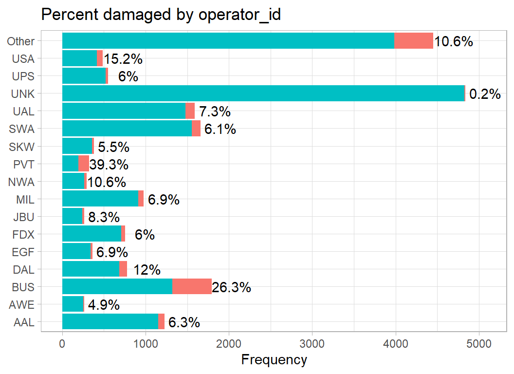
Business flights report more damage (26%) than average. The most common category is unknown (UNK), but when the operator is unknown, damage is rare.
aircraft_type distinguishes planes from helicopters.
# --- aircraft_type -----------------------------------------
trainRawDF %>%
  mutate( aircraft_type = factor(aircraft_type, levels=c("A", "B"),
                                 labels=c("Plane", "Helicopter"))) %>%
damage_plot(aircraft_type) 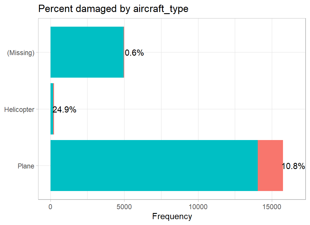
Most incidents are reported by planes but helicopters report damage on a higher percentage of flights. Missing data are common, but are rarely associated with damage. Presumably, pilots report more fully when the aircraft is damaged.
aircraft_mass describes the size of the aircraft, which ranges from single-seater planes up to jumbo jets. The labels are my own attempt to be more descriptive and are not in the database.
# --- aircraft_mass -----------------------------------------
trainRawDF %>%
  mutate( aircraft_mass = factor(aircraft_mass,
                                 levels=1:5,
                                 labels=c("single", "small", "medium",
                                 "large", "jumbo") )) %>%
damage_plot(aircraft_mass) 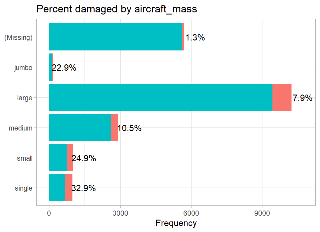
The high damage rate in the jumbos is surprising to me, though I would have anticipated the increased damage to small aircraft. Perhaps pilots of jumbos only notice wildlife strikes when they cause damage.
The number of engines is a value between 1 and 4.
# --- engines -----------------------------------------
trainRawDF %>%
  mutate( engines = factor(engines)) %>%
damage_plot(engines) 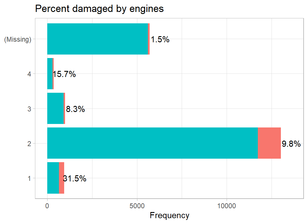
Probably the same story as we had for size of the aircraft, since large planes have more engines.
Engine type is just a letter code A to F. The letter distinguishes propellers from jet engines, but there are also turboprop and turbojets. Since I do not really understand these distinctions, I leave the codes as letters. A very few planes have more than one type of engine, for example “A/C”. When this happens I, rather arbitrarily, take the first letter. Just once in the whole dataset, the code is in lower case, so I correct that.
# --- engine_type -----------------------------------------
trainRawDF %>%
  mutate( engine_type = toupper(engine_type) ) %>%
  mutate( engine_type = substr(engine_type, 1, 1)) %>%
  mutate( engine_type = factor(engine_type)) %>%
damage_plot(engine_type) 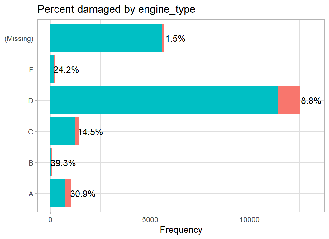
Obviously, jet engines are associated with larger planes so we may well be seeing the same pattern as with aircraft_mass
There are 4 codes showing the position of the engines. Presumably, the thought was that birds are more likely to fly into an engine suspended below the wing than they are to fly into an engine attached to the body of the plane. Engine position is a bit of a mess. Up to 4 engines are classified and by comparing numbers with aircraft types it looks to me as though the locations are 7=nose, 1,3,4=wing, 5=body, 6=tail and 2 is an unusual configuration in which the engine is more or less over the pilot’s head. The different wing codes probably distinguish positions within the wing, but it hard to be sure.
# --- position_code -----------------------------------------
trainRawDF %>%
  mutate( engine1_position = factor(engine1_position)) %>%
damage_plot(engine1_position) 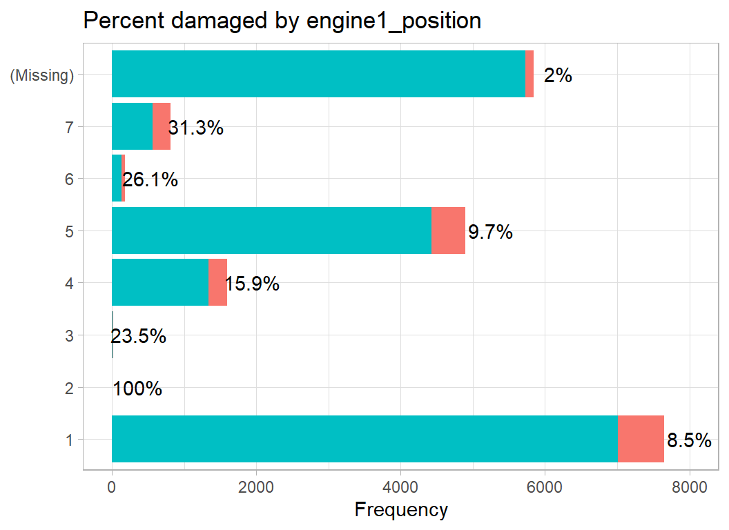
I will use operator_id, aircraft_type, aircraft_mass, engines, engine_type and a recoded version of position. The remainder will be dropped.
When coding indicator variables for the wing, nose, body and tail position of the engines there is problem with the missing values. If wing is missing then so will be nose, body and tail, it just reflects the fact that the engine positions are not available. When modelling, the missing values will be aliased with one another and the model would be over-parameterised. Good modelling software should cope with this, but I will remove the problem by only having a missing category for the wing variable.
The aircraft variables are cleaned with the following code and saved in a data frame called prep1DF, meaning the first preprocessed dataset.
# ==================================================================
# --- CLEAN THE AIRCRAFT VARIABLES ---------------------------------
#
# --- function for identifying for position codes ------------------
position_code <- function(thisDF, codes) {
  sum = 0
  for( c in codes) {
     sum = sum + (thisDF[, "engine1_position"] == c) +
                 (thisDF[, "engine2_position"] == c) +
                 (thisDF[, "engine3_position"] == c) +
                 (thisDF[, "engine4_position"] == c)
  }
  return( factor( as.numeric(sum > 0)) )
}

# --- cleaning code ------------------------------------------------
trainRawDF %>%
  # --- drop the variables that we don't want ----------------------
  select( -operator, -aircraft, -aircraft_make, -aircraft_model,
          -engine_make, -engine_model ) %>%
          # -------------- aircraft_mass ---------------------------
  mutate( aircraft_mass = factor(aircraft_mass, levels=1:5,
                                 labels=c("single", "small", "medium",
                                 "large", "jumbo") ),
          # -------------- aircraft_type ---------------------------
          aircraft_type = factor(aircraft_type, levels=c("A", "B"),
                                 labels=c("Plane", "Helicopter")),
          # -------------- engine_type -----------------------------
          engine_type = toupper(engine_type),
          engine_type = substr(engine_type, 1, 1),
          engine_type = factor( engine_type,
                                levels=c("A", "B", "C", "D", "F")),
          # --------------- engines ---------------------------------
          engines = factor(engines, levels=1:4),
          # -------------- operator_id ------------------------------
          operator_id = factor( operator_id),
          operator_id = fct_lump(operator_id, prop=0.01) ) %>%
  # --- code engine positions --------------------------------------
  replace_na( list(engine2_position=0, engine3_position=0,
                   engine4_position=0) ) %>%
  mutate( wing = position_code(., c(1, 3, 4))) %>%
  replace_na( list(engine1_position=0) ) %>%
  mutate( nose = position_code(., c(2, 7)),
          body = position_code(., 5),
          tail = position_code(., 6) ) %>%
  select( -contains("position") )  -> prep1DF
Time and Place
There are several variables that describe the location in time and space. We have the date as year, month and day, the visibility (day or night) the airport, the airport_id, the state and the faa_region.
To visualise the pattern over time, I’ve grouped the years into sets of three, otherwise the plot is rather crowded.
# --- years grouped into sets of three -------------------------
trainRawDF %>%
  mutate( year = 3*floor(incident_year/3) ) %>%
  mutate( year = factor(year)) %>%
damage_plot(year) 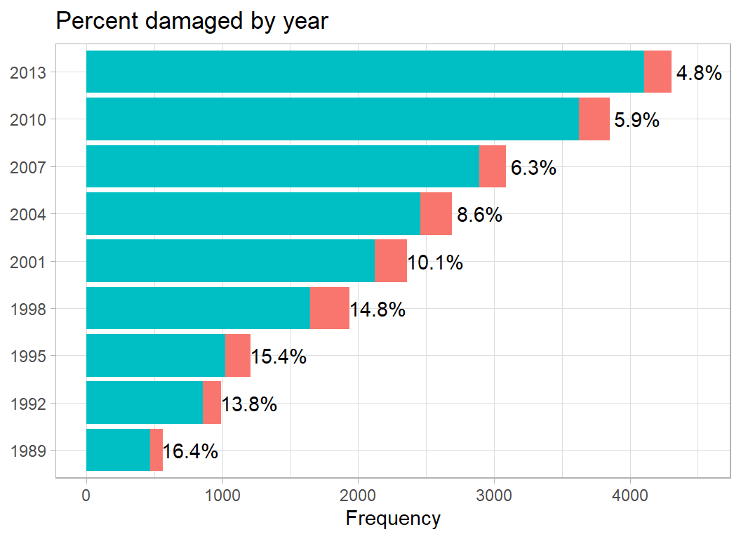
There is a clear pattern of increasing reports over time, but decreasing proportions of damage. This is typical of a reporting system that gradually becomes more complete. In the early years, reporting is less complete and the incident is much more likely to be reported when it is serious.
Here is the monthly pattern
# --- month ----------------------------------------------------
trainRawDF %>%
  mutate( month = factor(incident_month, labels=month.abb)) %>%
damage_plot(month) 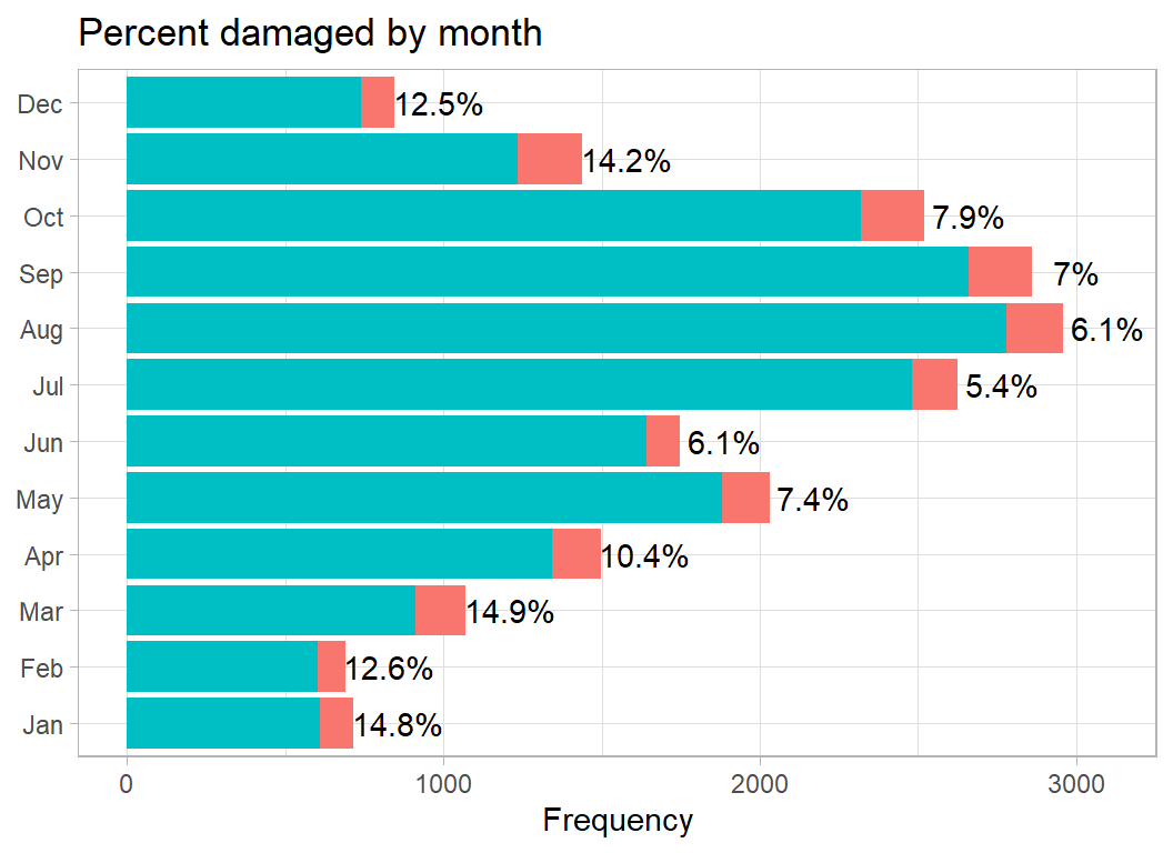
Fewer incidents in the winter but more damage when an incident occurs. Quite possibly, there are fewer flights in the winter.
Visibility, is the database’s slightly odd name for time of day.
# --- visibility (time of day) --------------------------------
trainRawDF %>%
  mutate( visibility = ifelse( visibility == "UNKNOWN", NA, visibility)) %>%
  mutate( visibility = factor(visibility)) %>%
damage_plot(visibility) 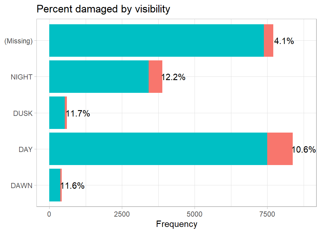
As we have seen with other variables, missingness is associated with less serious incidents. Otherwise, the percentage damaged is fairly steady.
A code of ZZZZ is used when the airport is not recorded. There are hundreds of airports, so I only plot the 10 most frequent.
# --- airport -----------------------------------------
trainRawDF %>%
  mutate( airport_id = ifelse( airport_id == "ZZZZ", NA, airport_id),
          airport_id = fct_lump_n(airport_id, n=10) ) %>%
damage_plot(airport_id) 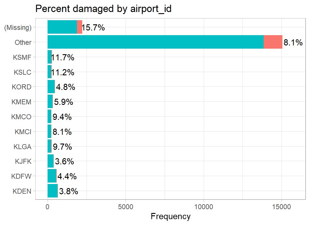
There are so many airports that the other category is huge. The percentage damaged seems fairly constant, although it is noticeably higher when the airport is missing. It seems unlikely that the airport is truly unknown, so it is quite likely that the missing airports are those outside the USA or they are incidents that did not take place close to an airport.
The FAA divides the USA into regions such as ANM = Northwest Mountain and ACE = Central. My guess is the other codes are made up for the database, for example, I assume that FGN = foreign.
# --- FAA region --------------------------------------
trainRawDF %>%
  mutate( faa_region = factor(faa_region) ) %>%
damage_plot(faa_region) 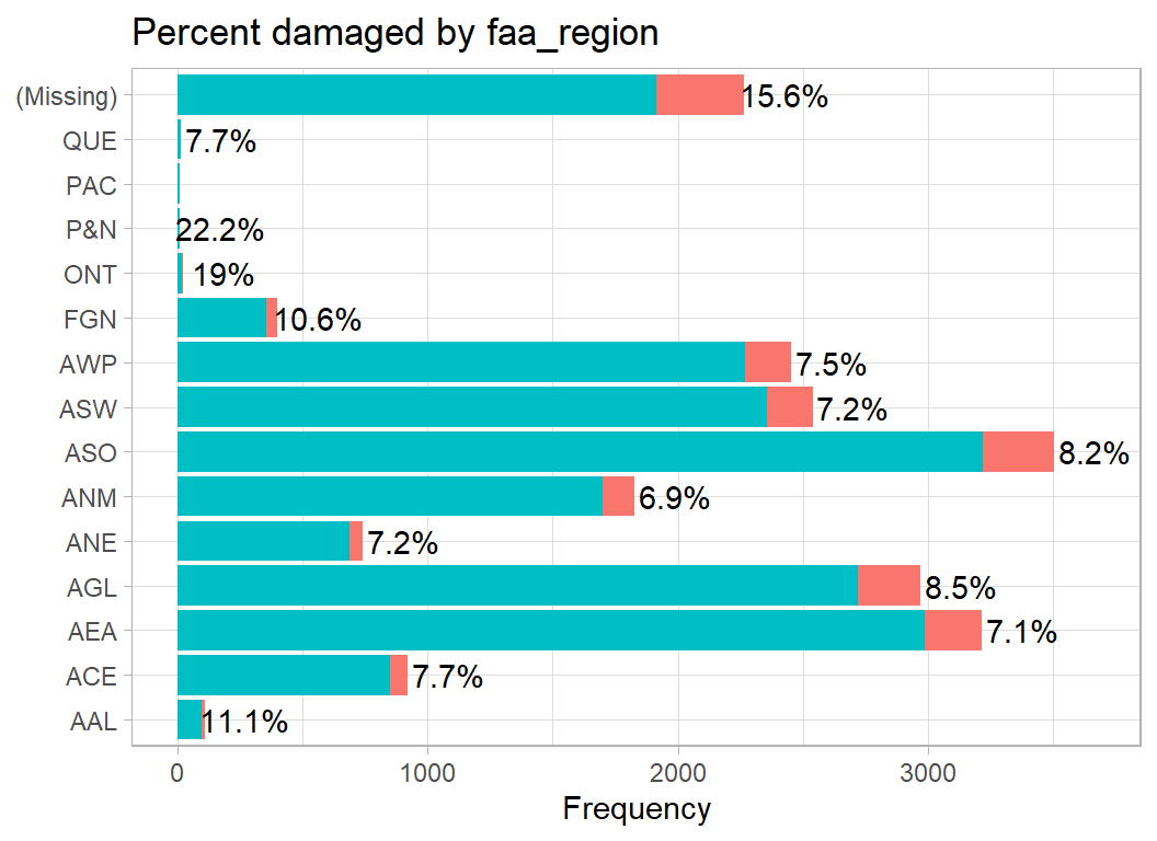
Damage seems to be more common in the smaller regions and when the region is missing.
In coding the locations, I ignore the airport and only use the FAA_regions. The results are saved in prep2DF
# ==================================================================
# --- CLEAN THE TIME & PLACE VARIABLES -----------------------------
#
prep1DF %>%
  # --- create a date variable -------------------------------------
  mutate( date = as.Date(paste(incident_year,
                               incident_month,
                               incident_day, sep="-"))) %>%
  select( -starts_with("inc")) %>%
  # --- recode visibility ------------------------------------------
  mutate( visibility = ifelse( visibility == "UNKNOWN", NA, visibility),
          visibility = factor( visibility, levels=c("DAWN",
                            "DAY", "DUSK", "NIGHT"))) %>%
  # --- recode faa_region ------------------------------------------
  mutate( faa_region = factor(faa_region),
          faa_region = fct_recode( faa_region,
                               FGN = "ONT", FGN = "P&N",
                               FGN = "PAC", FGN = "QUE") ) %>%
  # --- drop unwanted variables ------------------------------------
  select( - airport, -airport_id, -state) -> prep2DF
The wildlife
The size of the animal that the plane hits seems to me to be a key variable; hitting an moose is different from hitting a sparrow. Recoding the wildlife by size is time-consuming, but there is no real alternative.
I distinguish between small, medium and large animals and small, medium and large birds. The most common category is small birds, so I leave that as the default and list members of the other groups. My categorisation was obtained by looking through the entries and using my rather sketchy knowledge of American wildlife. The categorisation will not be perfect, but my hope is that it will be good enough.
This time I’ll clean the data first and then plot the resulting variables.
# ==================================================================
# --- CLEAN THE wildlife VARIABLES --------------------------------
#
# --- My categorisation of size ------------------------------------
# --- Small Animals ------------------------------------------------
smallAnimals <- c("BAT", "TERRAPIN", "TORTOISE")
# --- Medium Animals -----------------------------------------------
mediumAnimals <- c("OPOSSUM", "CAT", "DOG", "RABBIT", "MAMMAL", "TURTLE",
                   "COYOTE", "ARMADILLO", "BADGER", "SKUNK", "IGUANA",
                   "FOX", "MUSKRAT", "PORCUPINE", "RACCOON", "COTTONTAIL",
                   "OTTER", "WOODCHUCK", "MARMOT")
# --- Large Animals ------------------------------------------------
largeAnimals <- c("DEER", "ALLIGATOR", "ELK", "MOOSE")
# --- Medium Birds -------------------------------------------------
mediumBirds <- c("MEDIUM", "GULL", "OWL", "CROW", "KESTREL",
                 "HAWK", "FALCON", "DUCK", "UNKNOWN BIRD",
                 "RAVEN", "PIGEON", "MALLARD", "EIDER",
                 "TEAL", "GREBE", "MERLIN", "HARRIER", "GROUSE",
                 "CUCKOO", "CORMORANT", "PTARMIGAN", "PHEASANT",
                 "PINTAIL", "LOON", "GADWALL",
                 "ANHINGA", "BITTERN", "WIGEON",
                 "FULMAR", "MAGPIE", "SNIPE", "TERN", "WOODCOCK",
                 "SHOREBIRD", "SHEARWATER", "LAPWING", "RAIL")
# --- Large Birds -------------------------------------------------
largeBirds <- c("LARGE", "VULTURE", "GOOSE", "GEESE", "SWAN", "OSPREY",
                "TURKEY", "KITE", "STORK", "EAGLE", "PELICAN", "CRANE",
                "HERON", "EGRET", "FRIGATEBIRD", "IBIS")
# -----------------------------------------------------------------
# --- function to look for keywords -------------------------------
grade_size <- function(name, size, patternList, code) {
  for( x in patternList) {
    size <- ifelse( str_detect(name, x), code, size)
  }
  return(size)
}

# --- Grade size based on species_name ----------------------------
size <- rep("smallBird", nrow(trainRawDF))
name <- trainRawDF$species_name
size <- grade_size(name, size, largeAnimals,  "largeAnimal" )
size <- grade_size(name, size, mediumAnimals, "mediumAnimal" )
size <- grade_size(name, size, smallAnimals,  "smallAnimal" )
size <- grade_size(name, size, largeBirds,    "largeBird" )
size <- grade_size(name, size, mediumBirds,   "mediumBird" )

# --- Clean the tibble --------------------------------------------
prep2DF %>%
  mutate( size = factor(size) ) %>%
  select( -species_name, -species_id) %>%
  mutate( species_quantity = factor(species_quantity,
              levels=c("1", "2-10", "11-100", "Over 100"))) -> prep3DF
Now we can look at the effect of size of the wildlife.
# --- size of the wildlife ---------------------------------------
prep3DF %>%
damage_plot(size) 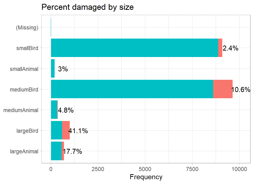
The number of animals is also critical, with a missing quantity being very similar to a strike by a single animal.
# --- number of birds/animals -------------------------------------
prep3DF %>%
damage_plot(species_quantity) 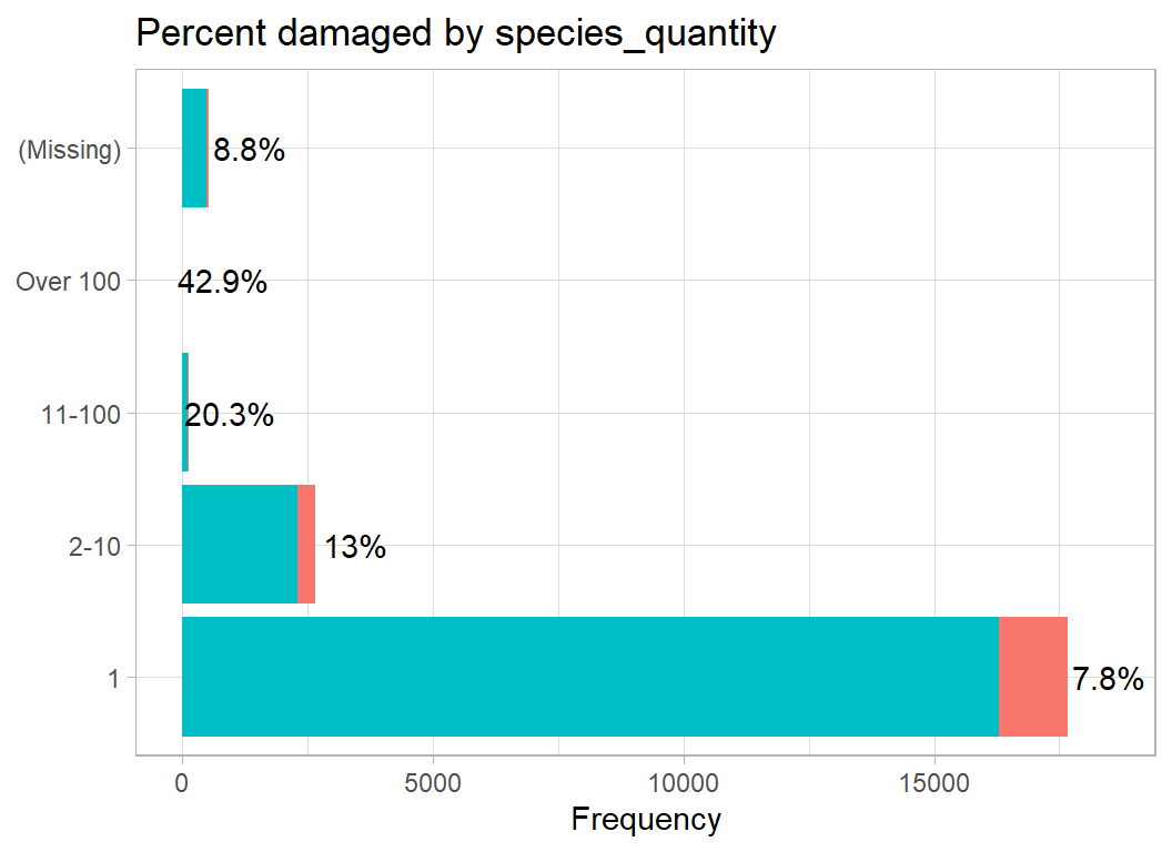
Conditions
The variables that describe the conditions at the time of impact are precipitation, height, speed, distance, flight_phase and flight_impact.
The height, speed and distance are poorly recorded and would require an elaborate imputation routine before they could be used. As we have seen with other variables, these measures are unlikely to be missing at random. I decided not to use them.
Precipitation classifies fog, rain and snow or a mix such as FOG/SNOW. I decided to create 3 indicator variables in place of precipitation in a similar way to engine position. We then have the same problem of over-parameterisation; the three are derived for the same source, so when fog is missing, rain and snow will also be missing. I put the missing category into fog.
The labels for impact on the flight are simplified and “SHUTDOWN” and “SHUT DOWN” with a space are combined into a single category. As with wildlife, I’ll clean first and plot second.
# ==================================================================
# --- CLEAN THE CONDITION VARIABLES --------------------------------
#
prep3DF %>%
  mutate( fog = as.numeric(str_detect(precipitation, "FOG")),
          fog = ifelse( is.na(precipitation), NA, fog),
          precipitation = ifelse( is.na(precipitation), "", precipitation),
          rain = as.numeric(str_detect(precipitation, "RAIN")),
          snow = as.numeric(str_detect(precipitation, "SNOW")),
          fog  = factor(fog),
          rain = factor(rain),
          snow = factor(snow)) %>%
  select( -precipitation) %>%
  mutate( flight_phase = ifelse( str_detect(flight_phase, "LAND"),
                                 "LANDING", flight_phase),
          flight_phase = ifelse( str_detect(flight_phase, "TAKEOFF"),
                                 "TAKEOFF", flight_phase),
          flight_phase = ifelse( str_detect(flight_phase, "LOCAL"),
                                 "PARKED", flight_phase),
          flight_phase = factor(flight_phase,
              levels=c("PARKED", "TAXI", "TAKEOFF",
                       "CLIMB", "EN ROUTE", "DESCENT",
                       "APPROACH", "LANDING")),
          flight_impact = ifelse( str_detect(flight_impact, "SHUT"),
                                 "SHUTDOWN", flight_impact),
          flight_impact = ifelse( str_detect(flight_impact, "ABORT"),
                                 "ABORT", flight_impact),
          flight_impact = ifelse( str_detect(flight_impact, "LAND"),
                                 "LANDING", flight_impact),
          flight_impact = factor(flight_impact)) %>%
  select( -height, - speed, -distance) -> prep4DF
Flight phase seems to suggest that the higher the altitude of the impact the more likely it is to cause damage.
# --- phase of the flight ---------------------------------
prep4DF %>%
  damage_plot(flight_phase)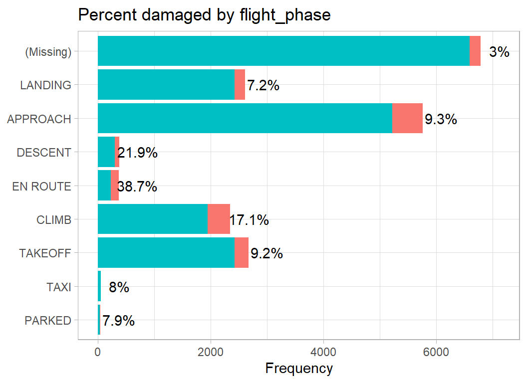
The impact on the flight is a good indicator of damage. In the rare cases where the pilot shuts down an engine, there is a very good chance that some damage has been caused.
# --- impact on the flight --------------------------------
prep4DF %>%
  damage_plot(flight_impact)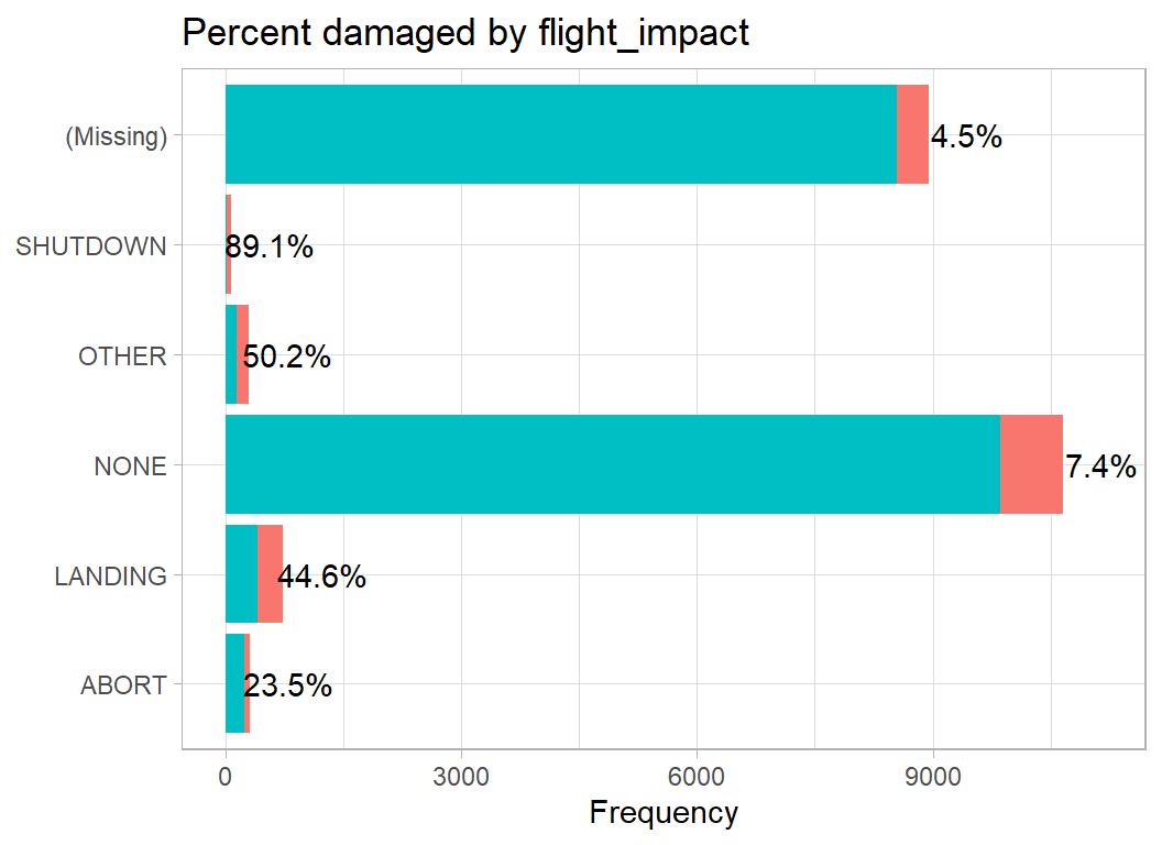
I am relatively happy with this data cleaning so the preprocessed data are saved for use in the modelling
# --- save the clean data ---------------------------------
prep4DF %>%
    saveRDS( file.path(home, "data/rData/clean_train.rds"))
Skim new dataset
The clean data are now ready for analysis, but as the changes are so extensive I summarise them
# --- skim the clean data ---------------------------------
skimr::skim(prep4DF)
As usual I have omitted the output from skim(). It is important to check it, but it is long and not very interesting.
What to do about missing data
Throughout the exploratory analysis we have seen that missingness is very informative. So imputation methods that ignore the response variable, damage are likely to perform very poorly. Yet, in the test data we do not have damage so we would be unable to impute properly in that dataset. Imputation would be a waste of effort. Instead, I will introduce a “missing” category to all of the factors and use “missing” as a potential predictor.
Logistic Regression
I’ll try a simple logistic model for the cleaned training data.
# ==================================================================
# --- Model the clean training data --------------------------------
#
library(broom)
library(lubridate)

# --- read clean data ----------------------------------------------
trainDF <-   readRDS( file.path(home, "data/rData/clean_train.rds"))

# --- fit logistic regression ---------------------------------------
trainDF %>%
  # --- extract year and month --------------------------------------
  mutate( yr = factor( year(date)),
          mth = factor( month(date))) %>%
  # --- introduce explicit missing categories -----------------------
  mutate( across(.cols=where(is.factor), .fns=fct_explicit_na) ) %>%
  # --- fit a logistic regression -----------------------------------
  glm( damaged ~ yr + mth + operator_id + aircraft_type +
         aircraft_mass + engines + engine_type + faa_region +
         flight_phase + visibility + species_quantity +
         flight_impact + nose + wing + body + tail + size +
         fog + rain + snow, data=., family="binomial") -> mod
Let’s look at the terms with a p-value below 0.01.
# --- model coefficients --------------------------------------------
tidy(mod) %>%
  filter( p.value < 0.01) %>%
  select( term, estimate, p.value) %>%
  print( n=80)
## # A tibble: 44 x 3
## term estimate p.value
## <chr> <dbl> <dbl>
## 1 yr1999 -0.672 6.03e- 3
## 2 yr2001 -0.801 1.04e- 3
## 3 yr2002 -0.938 1.35e- 4
## 4 yr2003 -0.870 4.37e- 4
## 5 yr2004 -0.842 7.14e- 4
## 6 yr2005 -1.11 1.16e- 5
## 7 yr2007 -0.728 2.90e- 3
## 8 yr2008 -1.15 1.57e- 5
## 9 yr2009 -1.12 1.26e- 5
## 10 yr2010 -0.834 7.90e- 4
## 11 yr2011 -1.09 1.53e- 5
## 12 yr2012 -1.05 2.45e- 5
## 13 yr2013 -0.740 2.60e- 3
## 14 yr2014 -1.49 3.21e- 9
## 15 yr2015 -1.09 3.31e- 5
## 16 mth5 -0.563 6.57e- 4
## 17 mth6 -0.507 4.08e- 3
## 18 mth7 -0.638 1.26e- 4
## 19 mth8 -0.611 1.48e- 4
## 20 mth9 -0.693 1.10e- 5
## 21 mth10 -0.606 1.24e- 4
## 22 operator_idBUS 0.785 3.13e- 5
## 23 operator_idDAL 0.668 3.44e- 4
## 24 operator_idPVT 0.975 1.35e- 4
## 25 operator_idUNK -1.86 3.14e- 5
## 26 operator_idUSA 0.808 7.68e- 5
## 27 aircraft_massmedium -0.994 1.89e- 6
## 28 aircraft_masslarge -1.50 1.83e-10
## 29 aircraft_mass(Missing) -2.35 4.66e- 4
## 30 engine_typeB 1.67 4.16e- 5
## 31 engine_typeD 0.828 1.97e- 4
## 32 faa_region(Missing) 1.94 8.55e- 6
## 33 flight_phaseDESCENT 2.40 4.34e- 3
## 34 species_quantity2-10 0.502 4.94e-10
## 35 species_quantity11-100 1.31 5.81e- 7
## 36 flight_impactLANDING 0.686 4.73e- 4
## 37 flight_impactNONE -1.02 1.80e- 8
## 38 flight_impactOTHER 0.842 2.16e- 4
## 39 flight_impactSHUTDOWN 3.09 2.38e-10
## 40 flight_impact(Missing) -0.876 5.80e- 6
## 41 sizemediumAnimal -1.31 2.14e- 5
## 42 sizemediumBird -1.18 4.38e-15
## 43 sizesmallAnimal -1.78 2.57e- 4
## 44 sizesmallBird -2.65 5.81e-59The factor, year, shows a large and consistent drop from 2002 onwards. A coefficient of -1 corresponds to a fall of over 60% in the proportion of damaged aircraft. This may be due to an increase in the number of minor incidents that are reported, rather than any true improvement.
The factor, month, shows a marked fall in the percentage of damaged aircraft during the summer months. Business (BUS) and Private (PVT) flights report more damage as do Delta and US airlines. When the operator is unknown (UNK) there are far fewer reports of damage.
Medium, large and missing aircraft sizes are associated with less damage. A missing FAA region is associated with more damage, perhaps because missing implies that the incident occurred outside the US borders. Quantity of animals is important in the way that might be expected. An engine shutdown has the strongest predictive effect of any feature. Small and medium size birds and animals do less damage than large ones.
We should also note the features that are not used by the model. Number of engines, aircraft_type (helicopter or plane), visibility (time of day), position of the engine, weather conditions.
Another way to look at the factors is through an analysis of deviance. In which we ask, does a factor such as operator_id show a relationship with damage? rather than ask about individual operators compared to some arbitrary base category.
In the analysis of deviance table, I’ve added a p-value and edited the layout slightly.
# --- analysis of deviance --------------------------------------
anova(mod) %>%
  { data.frame(term=rownames(.), .) } %>%
  as_tibble() %>%
  filter( term != "NULL" ) %>%
  mutate( p_value = pchisq(Deviance, df=Df, lower=FALSE)) %>%
  select( term, Df, Deviance, p_value) %>%
  print(n=20)
## # A tibble: 20 x 4
## term Df Deviance p_value
## <chr> <int> <dbl> <dbl>
## 1 yr 25 408. 7.27e- 71
## 2 mth 11 207. 2.17e- 38
## 3 operator_id 16 1355. 6.83e-279
## 4 aircraft_type 2 16.0 3.42e- 4
## 5 aircraft_mass 5 102. 2.36e- 20
## 6 engines 4 10.9 2.81e- 2
## 7 engine_type 5 18.9 1.99e- 3
## 8 faa_region 10 95.9 3.58e- 16
## 9 flight_phase 8 210. 5.82e- 41
## 10 visibility 4 18.5 9.84e- 4
## 11 species_quantity 4 56.6 1.53e- 11
## 12 flight_impact 5 730. 1.47e-155
## 13 nose 1 2.83 9.27e- 2
## 14 wing 2 14.0 8.92e- 4
## 15 body 1 2.26 1.33e- 1
## 16 tail 1 0.327 5.68e- 1
## 17 size 6 817. 2.93e-173
## 18 fog 2 3.01 2.22e- 1
## 19 rain 1 0.0617 8.04e- 1
## 20 snow 1 1.56 2.11e- 1The analysis of deviance confirms that weather conditions are not important and that only wing is significant amongst the engine positions. Wing is the feature that incorporates missing engine position.
To see how well the model predicts, we could start with the in-sample logloss, which is 0.195. Since the database is large and we have not done a lot of tuning this figure ought not be too misleading. I have deliberately not bothered to split the training data into an estimation and a validation set.
# --- insample logloss -----------------------------------------
trainDF %>%
  mutate( p = predict(mod, type="response") ) %>%
  summarise( logloss = -mean(damaged*log(p)+(1-damaged)*log(1-p)) )
## # A tibble: 1 x 1
## logloss
## <dbl>
## 1 0.195A useful way to assess goodness of fit of a logistic regression model is to make a plot based on the Hosmer-Leweshow statistic. The 21,000 incidents are divided into, say 20, bands based on their predicted probability of experiencing damage. Within these bands the observed and expected numbers of damaged aircraft are compared.
# --- 20 bands based on increasing risk ----------------------
broom::augment(mod, type.predict="response") %>%
  mutate( band = ntile(.fitted, 20)) %>%
    group_by( band) %>%
    summarise( n = n(),
               Observed = sum(damaged),
               Predicted = sum(.fitted),
               .groups="drop") %>%
    pivot_longer(Observed:Predicted,
                 names_to="class", values_to="value") %>%
    mutate( prob = value/n ) %>%
    ggplot( aes(x=band, y=prob, fill=class)) +
      geom_bar( stat="identity", position="dodge2") +
      scale_y_continuous( labels=scales::percent_format() ) +
      labs( y = "percent damaged", fill="") +
      scale_x_continuous( breaks=1:20 ) +
      labs(x="Risk bin", title="Hosmer-Lemeshow Plot") +
      theme( legend.position = c(0.1, 0.85))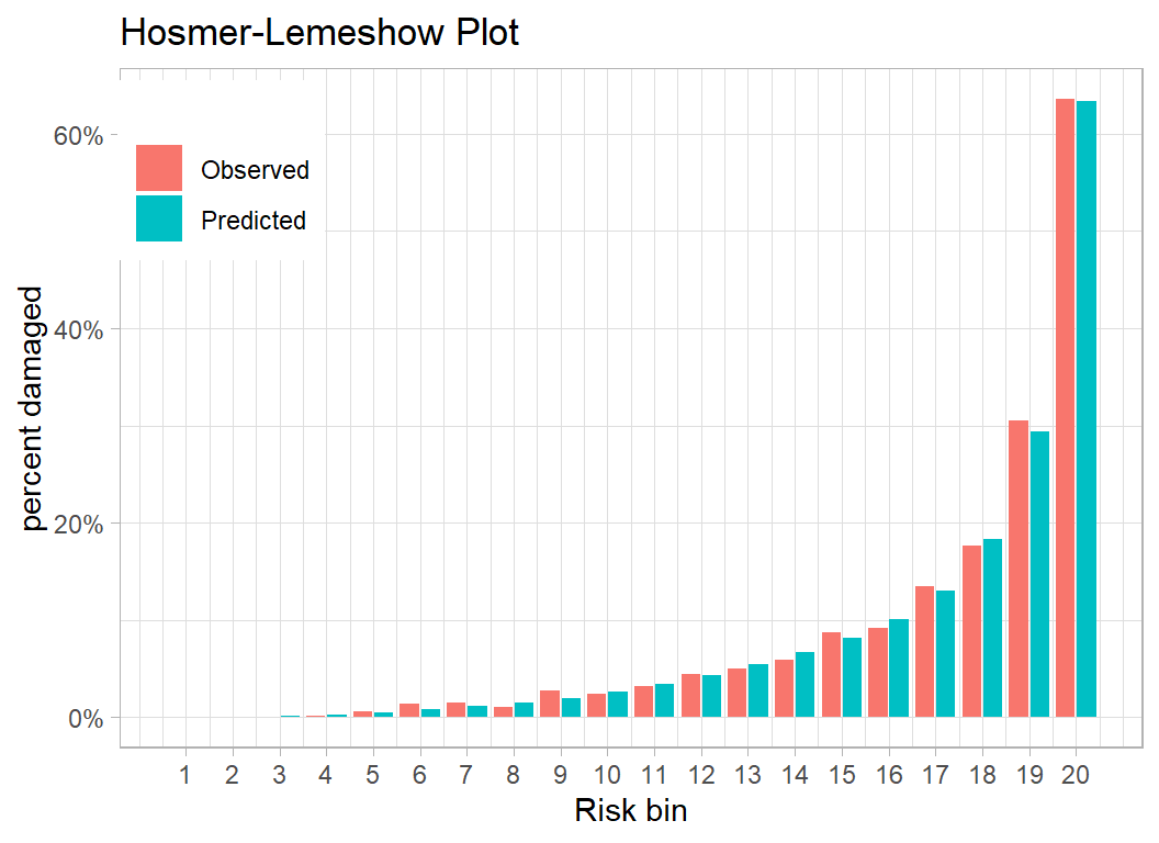
The model predicts very well and in the band with the highest 5% of predictions, we expect over 60% to report damage and almost exactly that percentage do.
We can compare observed and expected numbers using a chi-squared test
# --- Hosmer-Lemeshow statistic ---------------------------------
broom::augment(mod, type.predict="response") %>%
  mutate( band = ntile(.fitted, 20)) %>%
  # --- observed and expected numbers ---------------------------
  group_by( band ) %>%
  summarise( ExpDied = sum(.fitted),
             ObsDied = sum(damaged),
             ExpAlive = sum(1-.fitted),
             ObsAlive = sum(1-damaged)) %>%
  print() %>%
  # --- chi-squared test ----------------------------------------
  summarise( statistic =  sum( (ObsDied - ExpDied)^2/ExpDied ) +
               sum( (ObsAlive-ExpAlive)^2/ExpAlive ) ) %>%
  mutate( pvalue = pchisq(statistic, df=19, lower=FALSE))
## # A tibble: 20 x 5
## band ExpDied ObsDied ExpAlive ObsAlive
## <int> <dbl> <dbl> <dbl> <dbl>
## 1 1 0.302 0 1050. 1050
## 2 2 0.545 0 1049. 1050
## 3 3 1.27 0 1049. 1050
## 4 4 2.32 1 1048. 1049
## 5 5 5.16 6 1045. 1044
## 6 6 8.93 14 1041. 1036
## 7 7 12.3 16 1038. 1034
## 8 8 16.0 11 1034. 1039
## 9 9 21.0 29 1029. 1021
## 10 10 27.7 25 1022. 1025
## 11 11 35.8 34 1014. 1016
## 12 12 45.6 46 1004. 1004
## 13 13 56.7 52 993. 998
## 14 14 69.8 62 980. 988
## 15 15 85.4 92 965. 958
## 16 16 106. 96 944. 954
## 17 17 137. 142 913. 908
## 18 18 193. 185 857. 865
## 19 19 308. 320 742. 730
## 20 20 666. 668 384. 382## # A tibble: 1 x 2
## statistic pvalue
## <dbl> <dbl>
## 1 16.3 0.635As expected from the plot, the difference between observed and expected is not significant.
We could fit a slightly simpler model without the weather and most of the engine positions and we would expect performance to be similar.
# --- simplified logistic regression ---------------------------
trainDF %>%
  mutate( yr = factor( year(date)),
          mth = factor( month(date))) %>%
  mutate( across(.cols=where(is.factor), .fns=fct_explicit_na) ) %>%
  glm( damaged ~ yr + mth +
        operator_id + aircraft_type + aircraft_mass +
        engines + engine_type + faa_region + flight_phase +
        visibility + species_quantity + flight_impact +
        wing + size,
     data=.,
     family="binomial") -> mod

# --- in-sample logloss -----------------------------------------
trainDF %>%
  mutate( p = predict(mod, type="response") ) %>%
  summarise( logloss = -mean(damaged*log(p) + (1-damaged)*log(1-p)) )
## # A tibble: 1 x 1
## logloss
## <dbl>
## 1 0.196The in-sample logloss is very slightly worse at 0.196. Most statisticians would choose the simpler model, while I suspect that most people brought up in the Machine Learning tradition would prefer the full model.
I’m a statistician so I am drawn towards the simpler model, indeed I would be tempted to drop engines and visibility as well. On the other hand, I am also tempted to experiment with more operators.
To get a quick out-of-sample estimate of performance, I will fit the model to 80% of the data and measure performance on the other 20%. I’ll do this 5 times and average.
# --- prepare the data -----------------------------------------
trainDF %>%
  mutate( yr  = factor( year(date)),
          mth = factor( month(date))) %>%
  mutate( across(.cols=where(is.factor), .fns=fct_explicit_na) ) -> thisDF

# --- repeat five times ----------------------------------------
set.seed(8172)
logLoss <- rep(0, 5)
for( iter in 1:5 ) {
   # --- split the data ----------------------------------------
   split <- sample(1:21000, size=4200, replace=FALSE)

   validateDF <- thisDF[ split, ]
   estimateDF <- thisDF[-split, ]

   # --- fit to the training data ------------------------------
   estimateDF %>%
     glm( damaged ~ yr + mth +
            operator_id + aircraft_type + aircraft_mass +
            engines + engine_type + faa_region + flight_phase +
            visibility + species_quantity + flight_impact +
            wing + size,
     data=.,
     family="binomial") -> mod
   # --- logloss in validation set ----------------------------
   validateDF %>%
      mutate( p = predict(mod, type="response", newdata=. ) ) %>%
      summarise( logloss = -mean(damaged*log(p)+(1-damaged)*log(1-p)) ) %>%
      pull(logloss) -> logLoss[iter]

}
summary(logLoss)
## Min. 1st Qu. Median Mean 3rd Qu. Max.
## 0.1837 0.1856 0.1928 0.1966 0.1968 0.2242An we expected the mean cross-validated performance is very similar to the in-sample performance. If the logloss in the test data were to be 0.197, then the model would finish second on the leaderboard.
Submission
The last task is to clean the test set. In particular we must be careful to ensure that the factor operator_id has the same levels in the test data as it had when the training data were lumped, there is no guarantee that the most frequent operators in the test data will be the same as those in the training data.
There is a further problem in that the test data contain an FAA region, ATL, that does not appear in the training data. The frequency ATL is only 2, so I recode it as FGN.
# ======= CLEAN THE TEST SET ====================================

# --- categorise animal size ------------------------------------
size <- rep("smallBird", nrow(testRawDF))
name <- testRawDF$species_name
size <- grade_size(name, size, largeAnimals, "largeAnimal" )
size <- grade_size(name, size, mediumAnimals, "mediumAnimal" )
size <- grade_size(name, size, smallAnimals, "smallAnimal" )
size <- grade_size(name, size, largeBirds, "largeBird" )
size <- grade_size(name, size, mediumBirds, "mediumBird" )

# --- operator levels -------------------------------------------
op_levels <- levels(trainDF$operator_id)

# ==================================================================
# --- Clean the aircraft related variables -------------------------
#
testRawDF %>%
  # --- drop the variables that we don't want ----------------------
  select( -operator, -aircraft, -aircraft_make, -aircraft_model,
          -engine_make, -engine_model ) %>%
          # -------------- aircraft_mass ---------------------------
  mutate( aircraft_mass = factor(aircraft_mass, levels=1:5,
                                 labels=c("single", "small", "medium",
                                 "large", "jumbo") ),
          # -------------- aircraft_type ---------------------------
          aircraft_type = factor(aircraft_type, levels=c("A", "B"),
                                 labels=c("Plane", "Helicopter")),
          # -------------- engine_type -----------------------------
          engine_type = toupper(engine_type),
          engine_type = substr(engine_type, 1, 1),
          engine_type = factor( engine_type,
                                levels=c("A", "B", "C", "D", "F")),
         # --------------- engines ---------------------------------
         engines = factor(engines, levels=1:4),
         # -------------- operator_id ------------------------------
         operator_id = factor( operator_id, levels=op_levels),
         operator_id = fct_explicit_na(operator_id, na_level="Other") ) %>%
  # --- code engine positions --------------------------------------
  replace_na( list(engine2_position=0, engine3_position=0,
                   engine4_position=0) ) %>%
  mutate( wing = position_code(., c(1, 3, 4))) %>%
  replace_na( list(engine1_position=0) ) %>%
  mutate( nose = position_code(., c(2, 7)),
          body = position_code(., 5),
          tail = position_code(., 6) ) %>%
  select( -contains("position") ) %>%
# ==================================================================
# --- time and place ---------------------------------------------
# --- create a date variable -----------------------------------
  mutate( date = as.Date(paste(incident_year,
                               incident_month,
                               incident_day, sep="-"))) %>%
  select( -starts_with("inc")) %>%
  # --- recode visibility ------------------------------------------
  mutate( visibility = ifelse( visibility == "UNKNOWN", NA, visibility),
          visibility = factor( visibility, levels=c("DAWN",
                            "DAY", "DUSK", "NIGHT"))) %>%
  # --- recode faa_region ------------------------------------------
  mutate( faa_region = factor(faa_region),
          faa_region = fct_recode( faa_region, FGN = "ATL",
                               FGN = "ONT", FGN = "P&N",
                               FGN = "PAC", FGN = "QUE") ) %>%
  select( - airport, -airport_id, -state) %>%
# ==================================================================
# --- animal features ----------------------------------------------
#
  mutate( size = factor(size) ) %>%
  select( -species_name, -species_id) %>%
  mutate( species_quantity = factor(species_quantity,
              levels=c("1", "2-10", "11-100", "Over 100"))) %>%
# ==================================================================
# --- environmental variables --------------------------------------
#
  mutate( fog = as.numeric(str_detect(precipitation, "FOG")),
          fog = ifelse( is.na(precipitation), NA, fog),
          precipitation = ifelse( is.na(precipitation), "", precipitation),
          rain = as.numeric(str_detect(precipitation, "RAIN")),
          snow = as.numeric(str_detect(precipitation, "SNOW")),
          fog  = factor(fog),
          rain = factor(rain),
          snow = factor(snow)) %>%
  select( -precipitation) %>%
  mutate( flight_phase = ifelse( str_detect(flight_phase, "LAND"),
                                 "LANDING", flight_phase),
          flight_phase = ifelse( str_detect(flight_phase, "TAKEOFF"),
                                 "TAKEOFF", flight_phase),
          flight_phase = ifelse( str_detect(flight_phase, "LOCAL"),
                                 "PARKED", flight_phase),
          flight_phase = factor(flight_phase,
              levels=c("PARKED", "TAXI", "TAKEOFF",
                       "CLIMB", "EN ROUTE", "DESCENT",
                       "APPROACH", "LANDING")),
          flight_impact = ifelse( str_detect(flight_impact, "SHUT"),
                                 "SHUTDOWN", flight_impact),
          flight_impact = ifelse( str_detect(flight_impact, "ABORT"),
                                 "ABORT", flight_impact),
          flight_impact = ifelse( str_detect(flight_impact, "LAND"),
                                 "LANDING", flight_impact),
          flight_impact = factor(flight_impact)) %>%
  select( -height, - speed, -distance)  %>%
  saveRDS( file.path(home, "data/rData/clean_test.rds"))
Now we can make predictions using the reduced model fitted to the 21,000 training incidents. I need to refit the model to the training data then predict in the test set.
# --- Refit the reduced model ------------------------------------------
trainDF %>%
  mutate( yr = factor( year(date)),
          mth = factor( month(date))) %>%
  mutate( across(.cols=where(is.factor), .fns=fct_explicit_na) ) %>%
  glm( damaged ~ yr + mth +
          operator_id + aircraft_type + aircraft_mass +
          engines + engine_type + faa_region + flight_phase +
          visibility + species_quantity + flight_impact +
          wing + size,
     data=.,
     family="binomial") -> mod

# --- Read the cleaned test data --------------------------------------
readRDS( file.path(home, "data/rData/clean_test.rds")) %>%
  # --- create predictions --------------------------------------------
  mutate( yr = factor( year(date)),
          mth = factor( month(date)),
          across(.cols=where(is.factor), .fns=fct_explicit_na) ) %>%
  mutate( damaged= predict(mod, type="response", newdata=. ) ) %>%
  select( id, damaged) %>%
# --- write predictions to a csv file --------------------------------
  write.csv( file.path(home, "temp/submission1.csv"),
          row.names = FALSE)
When this file was submitted as a late submission on the kaggle website, the score was a logloss of 0.21067 on the private leaderboard (99% of the test data), very much in line with what we were expecting. This would have put us in sixth place on the leaderboard, where the best submission scored 0.19359.
I had a quick and not very systematic look at adding interactions and reducing the number of levels of some of the factors. It is easy to reduce the logloss to around 0.20, but some of the cells become very sparse, e.g. there are no privately run jumbo jets and the major carriers do not run single seater aircraft. Getting the logloss below 0.2 is much more of a challenge.
A tree-based model might improve on this level of performance because it could create interactions, say between the size of a bird and privately operated flights. This might work well for these data and for random splits of these data, but the results might not be very robust or be meaningful beyond this current dataset.
Given the amount of time spent on data cleaning, I will stop here.
What this example shows
I thought that this was a particularly tough example to use in a machine learning competition. The competitors would have been eager to get to the prediction models so as to ensure that they made some sort of submission, but really they needed to spend most of their time on unglamorous data cleaning.
The logistic regression model that I used in my analysis is very basic, but I had spent so much time on data cleaning that a adding complex model would have made this post indigestible. I am sure that Sliced will provide other problems that will be better vehicles for discussing classification models.
When you are presented with a messy set of data, you have two jobs to complete before you start modelling; you need to clean the data and you need to tidy the data. Cleaning is all about identifying and addressing inaccuracies in the data, while tidying involves organising the data in a structure suitable for analysis. Tidy data are organised in data frames, similar to the table of a relational database.
I think that the definition given by Wikipedia captures the essence of data cleaning,
“data cleaning is the process of detecting and correcting (or removing) corrupt or inaccurate records from a record set, table, or database and refers to identifying incomplete, incorrect, inaccurate or irrelevant parts of the data and then replacing, modifying, or deleting the dirty or coarse data”.
Perhaps the most interesting question that comes out of the analysis is, whether or not data cleaning is so problem specific that it is no scope for writing an R package that would help. dplyr, tidyr and forcats are very helpful and perhaps I should spend more time becoming familiar with their less well known functions, but I am left with the feeling that there is a gap in the tidyverse market.