Sliced Episode 8: Spotify Popularity
Summary
Background: In episode 8 of the 2021 series of Sliced, the competitors were given two hours in which to analyse a set of data on tracks available on Spotify. The aim was to predict the track popularity.
My approach: I merged the data on the tracks with data on the artists and then identified genres that were associated with the track popularity. Using all available information, I fitted a random forest model using default values of the hyperparameters.
Result: The RMSE of the model on the test data was 10.56, which placed the model in 4th place on the leaderboard.
Conclusion: The main problem was the time taken to fit the model, which effectively makes it impractical to tune the hyperparameters.
Introduction
The data for the eight episode of Sliced 2021 relate to tracks available on Spotify and can be downloaded from www.kaggle.com/c/sliced-s01e08-KJSEks. The data appear to be closely related to a much larger kaggle datset that is available from www.kaggle.com/yamaerenay/spotify-dataset-19212020-160k-tracks. The task for the contestants was to build a model that predicts the popularity of a track.
Popularity is a number between 0 and 100 that is based on a track’s recent plays. Spotify uses the popularity when it recommends tracks or creates playlists. The algorithm used to measure popularity has not been made public, nor is it clear how often the popularity score is updated. As popularity depends on recent plays, it can decrease if a track is played less often than it used to be, and because popularity is not updated in real time, there may be a lag before new tracks get a popularity score that truly reflects the number of times that they are being played.
I thought that these data would be a good vehicle for investigating random forests, although first there will be a good deal of feature extraction.
Reading the Data
It is my practice to read the data asis and to immediately save it in rds format within a directory called data/rData. For details of the way that I organise my analyses you should read my post called Sliced Methods Overview.
For this episode there was a second file of data on artists that includes a short description of their genre and a measure of the artists popularity. Not every artist with a track in the training set is present in the artist file, but most are.
# --- setup the libraries etc. ---------------------------------
library(tidyverse)

theme_set( theme_light())

# --- the project folder ---------------------------------------
home  <- "C:/Projects/kaggle/sliced/s01-e08"

# --- read the training data -----------------------------------
trainRawDF <- readRDS( file.path(home, "data/rData/train.rds"))

# --- read the data on the artists -----------------------------
artistRawDF <- readRDS( file.path(home, "data/rData/artists.rds"))

# --- read the test data ---------------------------------------
testRawDF <- readRDS( file.path(home, "data/rData/test.rds"))
As usual I start by running skim() to look at the structure of the data, but I hide the output because it is long and would interrupt the flow.
# --- summarise training data with skimr -----------------------
skimr::skim(trainRawDF)

skimr::skim(artistRawDF)
skim() shows that there are 21,000 tracks in the training data. There is no missing data problem apart from release month/day that is missing for about a quarter of the tracks.
The artists file has information on 17,718 artists including the popularity of the artist (as opposed to the popularity of a track) and text on the genre of the artist.
The response
The response is track popularity; it has an average of 27.6 and as the histogram shows it has a bimodal distribution with one mode at zero and another around 35.
# --- histogram of track popularity ---------------------------
trainRawDF %>%
  ggplot(aes(x=popularity) ) +
  geom_histogram( binwidth=1, fill="steelblue") +
  labs(title="Track popularity on Spotify")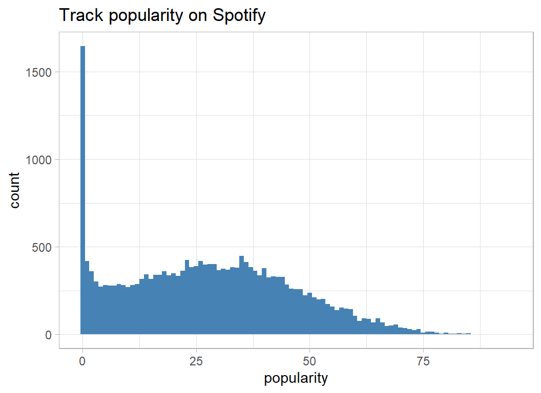
A regression model would have two problems; one due to the bimodality and the other due to the limits on the range, especially the boundary at a zero. So, it is a good thing that I decided to try random forests.
The “proper” way to handle bimodality is with a mixture model that assigns tracks to one or other of the distributions and has separate prediction equations for each distribution. The data would be a good vehicle for showing how stan can be used to fit a Bayesian mixture model.
Predictors
track variables
The code needed for looking at the various continuous predictors in very repetitive, so I’ve turned it into a function. Since there are so many potential data points, I’ve chosen to use geom_hex to show the count within a given hexagonal regions of the plot.
plot_hexes <- function(thisDF, col) {
  thisDF %>%
  ggplot( aes(x=.data[[col]], y=popularity)) +
  geom_hex( bins=50) +
  geom_smooth( colour="red", fill="darkorange") +
  lims( y=c(0,100)) +
  labs( title=paste("Popularity by track", col)) +
  scale_fill_viridis_c(trans="log10")
}
Duration is measured in milliseconds and has a large range that argues for a log transformation. The other predictors have been left on their original scales.
Very short and very long tracks are least popular.
trainRawDF %>%
  mutate( duration = log10(duration_ms / 1000)) %>%
  plot_hexes("duration")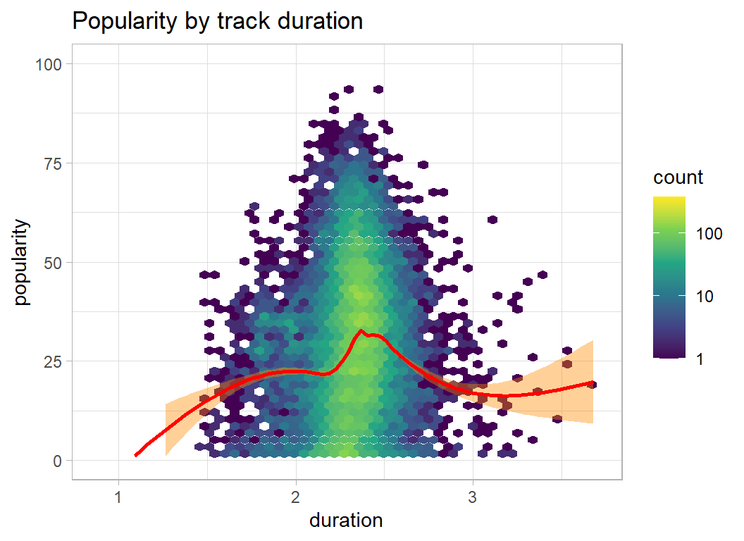
I give the other plots and then summarise what they show
trainRawDF %>%
  plot_hexes("danceability")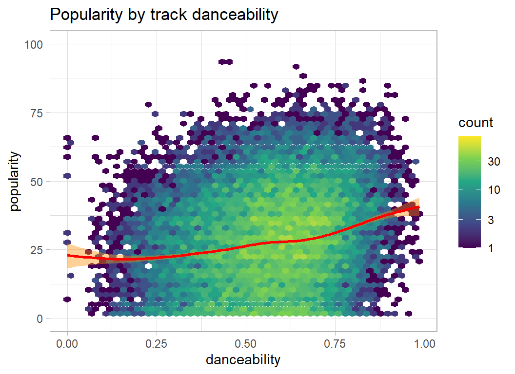
trainRawDF %>%
  plot_hexes("energy")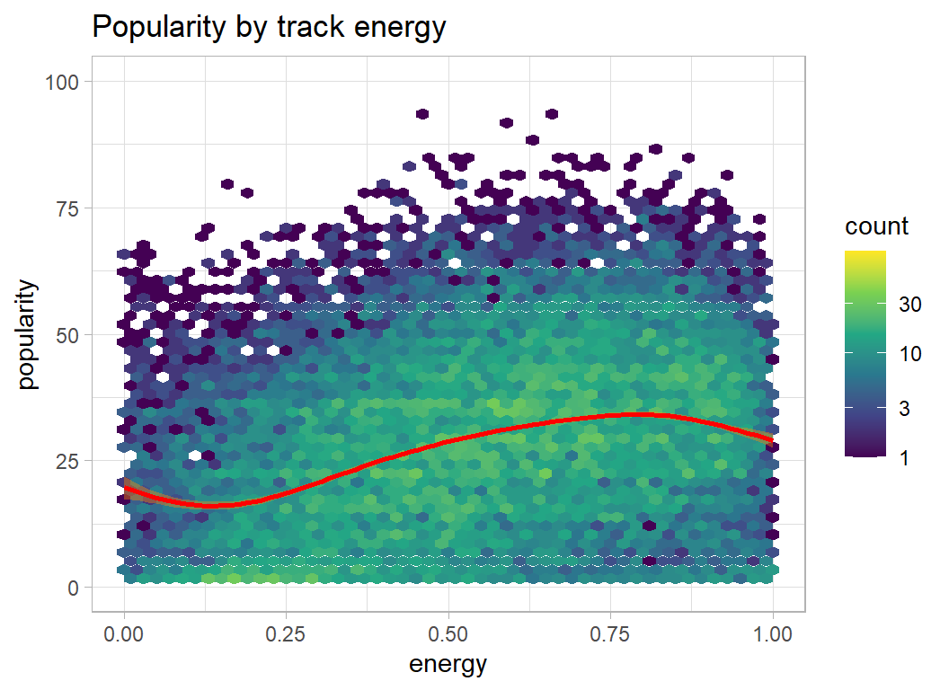
trainRawDF %>%
  plot_hexes("loudness")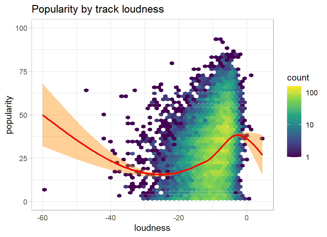
trainRawDF %>%
  plot_hexes("speechiness")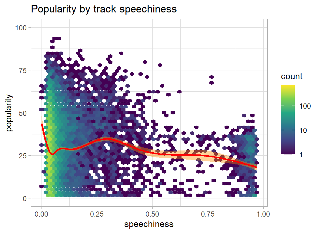
trainRawDF %>%
  plot_hexes("acousticness")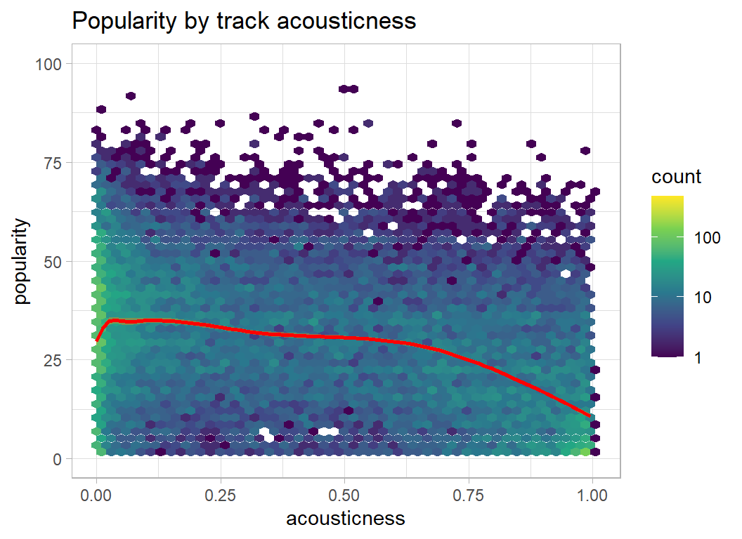
trainRawDF %>%
  plot_hexes("liveness")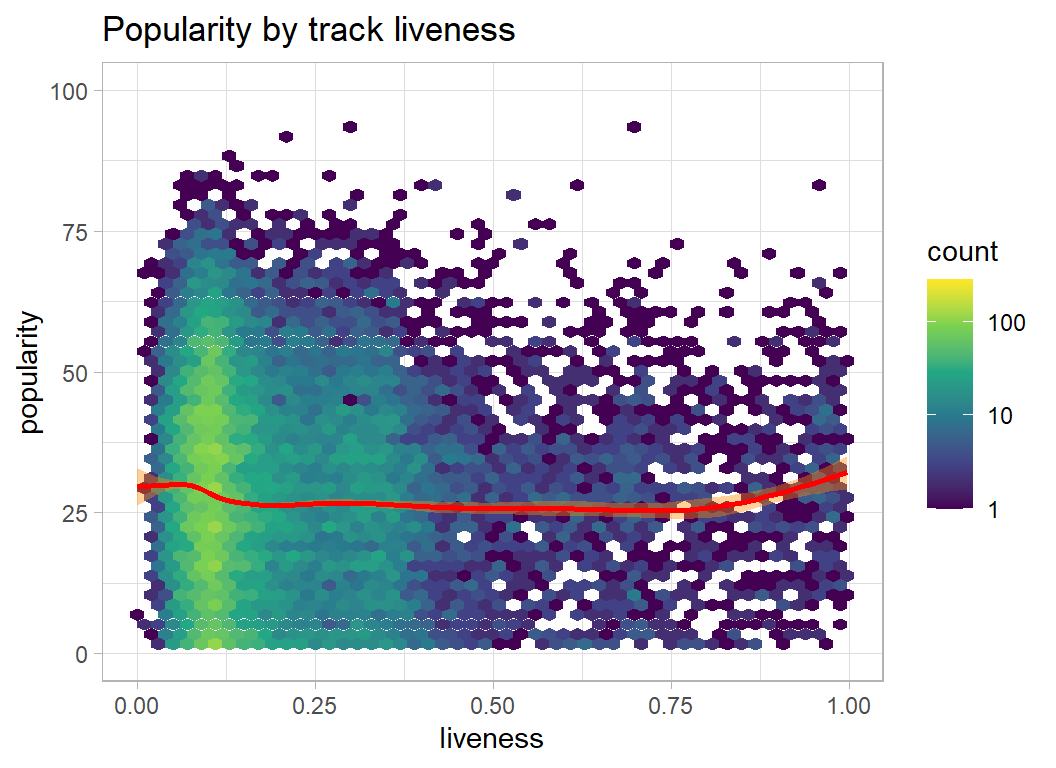
trainRawDF %>%
  plot_hexes("instrumentalness")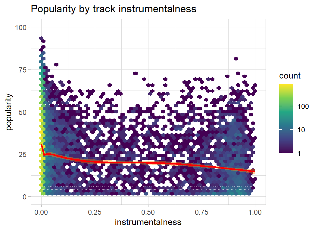
trainRawDF %>%
  plot_hexes("valence")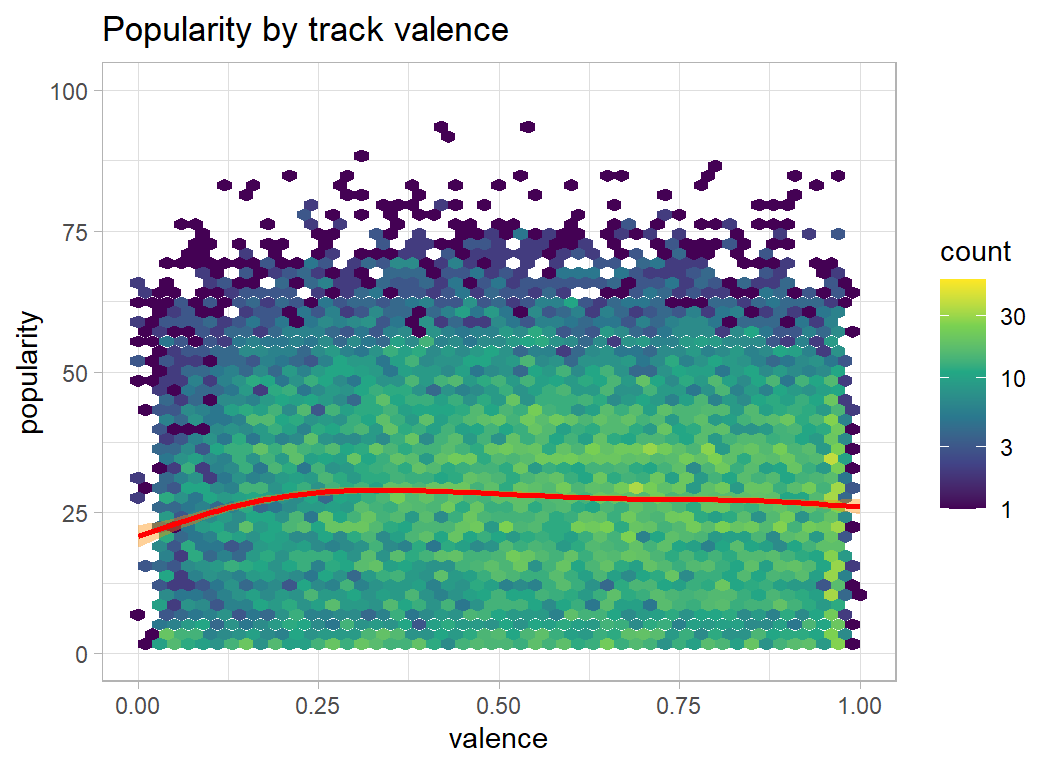
trainRawDF %>%
  plot_hexes("tempo")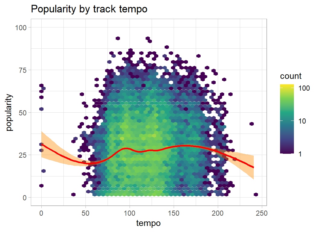
trainRawDF %>%
  plot_hexes("release_year")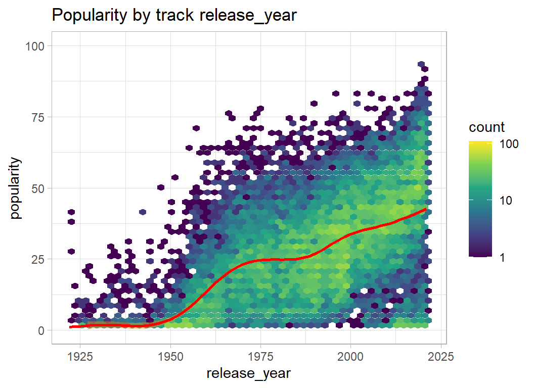
Here is my summary of what the plots show
- danceability, energy, loudness … the higher the better
- speechiness, acousticness, liveness, instrumentalness … the lower the better
- valence, tempo … no clear relationship with popularity
- release_year … very strong preference for recent years
Artists
Much like the track popularity, the artist popularity is a bimodal distribution, but with one mode at zero and another around 45.
# --- artist popularity ---------------------------------------
artistRawDF %>%
  ggplot(aes(x=popularity) ) +
  geom_histogram( binwidth=1, fill="steelblue") +
  labs(title="Artist popularity on Spotify")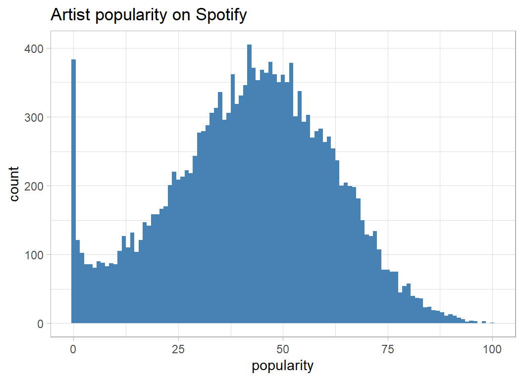
Followers are users of Spotify who click to say that they follow a particular artist. Building up the number of followers is important for artists because it helps get their tracks onto playlists.
Naturally enough, the number of followers is related to an artists popularity (plays).
artistRawDF %>%
  ggplot( aes(x=log10(followers+1), y=popularity )) +
  geom_hex( bins=50) +
  geom_smooth( colour="red", fill="darkorange") +
  lims( y=c(0,100)) +
  labs( title="Artist's popularity by followers") +
  scale_fill_viridis_c(trans="log10")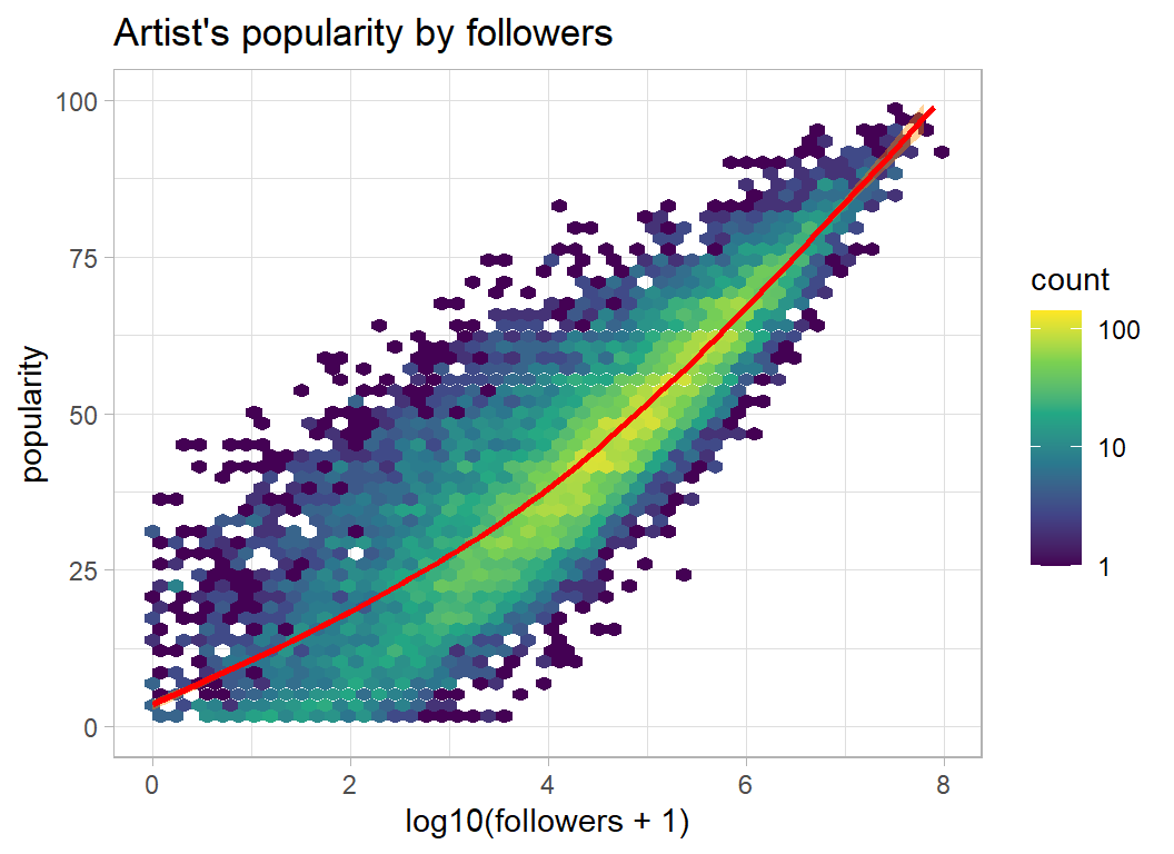
Artist’s genres
The artists are classified by the genre of their music. Here are some examples,
artistRawDF %>%
  select( genres) %>%
  print()
## # A tibble: 17,718 x 1
## genres
## <chr>
## 1 ['country blues', 'country rock', 'piedmont blues']
## 2 ['turkish pop']
## 3 ['celtic', 'irish folk']
## 4 ['kindermusik', 'kleine hoerspiel']
## 5 ['opm', 'vispop']
## 6 ['classic mandopop']
## 7 ['album rock', 'alternative rock', 'blues rock', 'classic rock', 'country ro~
## 8 ['country', 'country rock', 'oklahoma country']
## 9 ['trondersk musikk']
## 10 ['alternative rock', 'anti-folk', 'indie rock', 'modern rock', 'permanent wa~
## # ... with 17,708 more rowsMerging artists and tracks
I want to associate the genres of the artist with their tracks. This does not guarantee that the genre will refer to that track. It just means that the artist who produced the track usually works in that genre.
There is one extra problem, some tracks have multiple artists. I only take the first two artists for any track and I take the average popularity and average number of followers of the artists plus their combined list of genres. This means that third and fourth artists will be ignored.
# --- merge artist data into the track file --------------------------
trainRawDF %>%
  # --- remove extra characters from id_artists -------------------
  mutate( id_artists = str_replace_all(id_artists, "\\'", "")) %>%
  mutate( id_artists = str_replace_all(id_artists, "\\[", "")) %>%
  mutate( id_artists = str_replace_all(id_artists, "\\]", "")) %>%
  # --- extract first two artists --------------------------------
  separate(id_artists, into=c("artistId1", "artistId2"),
           sep=",", extra="drop") %>%
  # --- merge first artist ---------------------------------------
  mutate( id_artists = artistId1 ) %>%
     left_join(artistRawDF %>%
                  rename( id_artists = id,
                          follow1    = followers,
                          popArtist1 = popularity) %>%
                  select(id_artists, genres, popArtist1, follow1),
               by = "id_artists")  %>%
  rename( genre1 = genres ) %>%
  mutate( genre1 = ifelse( is.na(genre1), "", genre1 )) %>%
  # --- merge second artist --------------------------------------
  mutate( id_artists = artistId2 ) %>%
  left_join(artistRawDF %>%
               rename( id_artists = id,
                       follow2    = followers,
                       popArtist2 = popularity) %>%
               select(id_artists, genres, popArtist2, follow2),
            by = "id_artists") %>%
  rename( genre2 = genres ) %>%
  mutate( genre2 = ifelse( is.na(genre2), "", genre2 )) %>%
  # --- combine the genres ---------------------------------------
  unite( genre, genre1, genre2,  sep="," ) %>%
  # --- average popularity & followers ---------------------------
  rowwise() %>%
  mutate( avgArtistPop = mean( c(popArtist1, popArtist2),
                              na.rm=TRUE),
          avgFollowers = mean( c(follow1, follow2),
                              na.rm=TRUE) ) %>%
  mutate( avgArtistPop = ifelse( is.nan(avgArtistPop),
                                 NA, avgArtistPop),
          avgFollowers = ifelse( is.nan(avgFollowers),
                                 NA, avgFollowers)) %>%
  # --- drop working variables -----------------------------------
  ungroup() %>%
  select( -artistId1, -artistId2, -popArtist1, -popArtist2,
          -follow1, -follow2, -id_artists)  -> prep1DF
Popular genres
Now that genres are associated with tracks we can look for commonly occurring terms that are associated with track popularity. I have done something similar for several of the Sliced datasets using code that I gave in episode 1. I’ll use the same function, select_indicators(), for these data.
I’ll start by removing the square brackets from genre and then I’ll split using the commas.
library(myText)

prep1DF %>%
  mutate( genre = str_replace_all(genre, "\\[", ""),
          genre = str_replace_all(genre, "\\]", ""),
          genre = ifelse( is.na(genre), "", genre )) %>%
  select_indicators(col=genre, response=popularity,
                    nTerms=12, minCount=100, sep=",") %>%
  filter( p_value < 0.001 ) %>%
  print(n=10) -> wordsDF
## # A tibble: 130 x 5
## term count p_value mWithout mWith
## <chr> <int> <dbl> <dbl> <dbl>
## 1 'classical' 656 4.84e-151 28.2 9.75
## 2 'rock' 1143 4.16e-108 27.0 37.6
## 3 'pop' 378 3.87e- 93 27.1 54.6
## 4 'dance pop' 389 8.19e- 89 27.2 50.4
## 5 'vintage tango' 109 4.48e- 78 27.7 1.05
## 6 'classic bollywood' 380 6.24e- 69 27.8 13.3
## 7 'classic icelandic pop' 144 2.04e- 68 27.7 8.63
## 8 'tango' 115 2.19e- 68 27.7 1.84
## 9 'rap' 175 4.87e- 64 27.3 55.2
## 10 'hip hop' 177 1.74e- 63 27.4 53.1
## # ... with 120 more rows‘classical’ tracks are not popular but ‘rock’ tracks are. Notice however, that ‘rock’ is different from ‘classic rock’ or ‘soft rock’ and countless other types of rock.
I make indicator variables for the 130 chosen words and at the same time I create an indicator variables for the key, which ranges from 1 to 11
# --- indicators for the top genres -------------------------------
prep1DF <- add_indicators(prep1DF, "genre", wordsDF$term, "X")

# --- indicators for the keys -------------------------------------
prep1DF <- add_indicators(prep1DF, "key", as.character(1:11), "K")
Zeros & missing values
Many of the continuous measures contain a few zeros that are well separated from the bulk of the scores. Let’s take speechiness as an example
prep1DF %>%
  filter( speechiness == 0 ) %>%
  select(popularity, avgArtistPop, name) %>%
  print( n=10 )
## # A tibble: 18 x 3
## popularity avgArtistPop name
## <int> <dbl> <chr>
## 1 52 NA "White Noise Car Sound for Baby Sleep (Loopable)"
## 2 7 59 "Wus Geven Ist Geven"
## 3 64 NA "Big Fan Dulled"
## 4 27 76 "Kapitel 37 - als Bürgermeister (Folge 057)"
## 5 53 NA "Staubsauger (Sanft)"
## 6 65 NA "White Noise for Baby 432 Hz (Loopable with No Fade)"
## 7 32 NA "Rain Sounds & White Noise (Loopable, No Fade Sleep ~
## 8 0 47 "El amor brujo \"Ballet-pantomime\": 4. El Aparecido"
## 9 32 NA "Heavier Rain Fall with Thunder"
## 10 28 31 "Sleeping Baby One Hour of Pink Noise"
## # ... with 8 more rowsSome are white noise tracks that are amazingly popular. Staubsauger is the German for vacuum cleaner, so the lack of speechiness seems real, even if the popularity is a mystery. These zeros look genuine to me and I’ll leave them asis.
We do have some cases where the artists in trainRawDF are not in the artistRawDF. Presumably, these are recordings by lesser known artists or unidentified artists. When this happens there will not be any genre information.
A sensible policy would be to impute the popularity of the missing artists from the popularity of their tracks, but of course we would not be able to do that for the test data because the track popularity is missing. Instead, I decided to impute using the median popularity of the tracks of unknown artists
# --- median track popularity when there is no data on the artist ---
prep1DF %>%
  filter( is.na(avgArtistPop) ) %>%
  summarise( mPop = median(popularity))
## # A tibble: 1 x 1
## mPop
## <int>
## 1 6So the typical track popularity when the artist is missing from the artists file is 6.
I will also introduce an extra indicator, artistNA, to denote missing artists in case that is predictive.
# --- impute missing values -----------------------------------------
prep1DF %>%
  mutate( artistNA = as.numeric( is.na(avgArtistPop)),
          avgArtistPop = ifelse(is.na(avgArtistPop), 6, avgArtistPop ),
          avgFollowers = ifelse(is.na(avgFollowers), 0, avgFollowers ))  -> prep1DF
The names of the tracks are unlikely to contain much useful information. Here are some examples,
prep1DF %>%
  select(name)
## # A tibble: 21,000 x 1
## name
## <chr>
## 1 blun7 a swishland
## 2 Que Me Perdone Tu Señora
## 3 愛唄~since 2007~
## 4 Let me be your uncle tonight
## 5 Never Going Back Again - 2004 Remaster
## 6 Lilla snigel
## 7 Meu Lugar
## 8 Khalifa
## 9 From Four Until Late
## 10 Riders On the Storm
## # ... with 20,990 more rowsIt would be interesting to identify the language, but that would involve far too much work. So, let’s just look for informative words. I start by converting to lower cases and dropping anything that is not alphabetic. Then I only keep words with more than 2 characters.
prep1DF %>%
  mutate( name = tolower(name),
          name = str_replace_all(name, "[^a-z]", " ") ) %>%
  select_indicators(col=name, response=popularity,
                    nTerms=12, minCount=100, sep=" ") %>%
  filter( p_value < 0.001 ) %>%
  filter( str_length(term) > 2 ) %>%
  print(n=20) -> wordsNameDF
## # A tibble: 19 x 5
## term count p_value mWithout mWith
## <chr> <int> <dbl> <dbl> <dbl>
## 1 feat 270 3.84e-47 27.3 46.9
## 2 chapter 80 1.70e-42 27.7 1.98
## 3 remasterizado 123 1.20e-33 27.7 5.56
## 4 act 169 9.99e-33 27.7 10.2
## 5 major 134 1.21e-30 27.7 9.51
## 6 folge 179 6.32e-28 27.5 31.6
## 7 blues 125 1.83e-27 27.7 11.1
## 8 vivo 133 1.88e-22 27.5 42.6
## 9 remaster 931 1.39e-13 27.8 23.2
## 10 mix 425 2.93e-12 27.7 20.4
## 11 all 667 4.52e- 6 27.7 24.2
## 12 original 119 6.30e- 6 27.6 19.0
## 13 and 846 3.26e- 5 27.7 24.8
## 14 amor 194 4.96e- 5 27.5 32.8
## 15 die 269 5.94e- 5 27.6 23.5
## 16 kapitel 265 7.62e- 5 27.6 24.4
## 17 live 426 1.45e- 4 27.6 24.7
## 18 take 136 6.60e- 4 27.6 22.4
## 19 del 215 9.47e- 4 27.6 23.9Only 19 words look informative.
remaster and remasterizado seem to identify the same type of track. mix and original are also generic terms. chapter picks out audio books. act and major probably identify classical tracks. Google tells me that feat refers to featuring, as in “artist A featuring artist B” (something tells me that I am one of the few people in the world who didn’t already know that). folge seems to pick out German tracks, I think that it means episode. folge is often found together with kapitel, the German for chapter.
My selection is very subjective. I assumed that the classical terms would be picked by by the genre.
# --- my selection of important words ------------------------
myWords <- c("remaster", "mix", "original", "chapter", "feat")

# --- remove missing values from name ------------------------
prep1DF$name <- ifelse( is.na(prep1DF$name), "", prep1DF$name)

# --- add indicator variables --------------------------------
prep1DF <- add_indicators(prep1DF, "name", myWords, "N")
Finally I’ll rescale duration_ms and add indicators for the last 4 months before the end of the period of data collection. I do this in base R because my add_indicators() function was not written for pairs of conditions
# --- rescale duration ---------------------------------------
prep1DF$duration <- log10(prep1DF$duration_ms/1000)

# --- replace missing months with zero -----------------------
prep1DF$release_month <- ifelse( is.na(prep1DF$release_month), 0, prep1DF$release_month)

# make indicators for the last 4 months ----------------------
for( i in 1:4) {
  prep1DF[ paste("M", i, sep="") ] <- as.numeric(prep1DF$release_month == i & prep1DF$release_year == 2021 )
}

# --- save the pre-processed data ----------------------------
saveRDS( prep1DF, file.path(home, "data/rData/processed_train.rds"))
Predictive models
I decided to use these data to illustrate random forests.
There is a small problem with these data; we have 12 continuous predictors and 151 indicators (130 from genre, 11 from key, artistNA, M1 to M4 and 5 from name), plus there are 21,000 tracks. It is going to be slow.
The randomForest package likes the data in matrices, so I’ll start by splitting the data into an estimation (n=13000) and a validation (n=8000) set and then I’ll extract the necessary matrices.
library(randomForest)

# --- read the processed training data ------------------------------
trainDF <- readRDS(file.path(home, "data/rData/processed_train.rds"))

# --- split into estimation and validation --------------------------
set.seed(6671)
split <- sample(1:21000, size=8000, replace=FALSE)

# --- response for the estimation set -------------------------------
trainDF %>%
  slice(-split) %>%
  pull(popularity) -> Y

# --- predictors for the estimation set -----------------------------
trainDF %>%
  slice(-split) %>%
  select( duration, danceability, energy, loudness, speechiness,
  acousticness, liveness, valence, tempo, instrumentalness,
  avgArtistPop, avgFollowers, release_year, artistNA, M1, M2, M3, M4,
  starts_with("X", ignore.case=FALSE),
  starts_with("N", ignore.case=FALSE),
  starts_with("K", ignore.case=FALSE))  %>%
  as.matrix() -> X


# --- predictors for the validation set ----------------------------
trainDF %>%
  slice(split) %>%
  select( duration, danceability, energy, loudness, speechiness,
  acousticness, liveness, valence, tempo, instrumentalness,
  avgArtistPop, avgFollowers, release_year, artistNA, M1, M2, M3, M4,
  starts_with("X", ignore.case=FALSE),
  starts_with("N", ignore.case=FALSE),
  starts_with("K", ignore.case=FALSE))  %>%
  as.matrix() -> XV
Now we can fit a random forest using the package defaults. It takes a while (about 10minutes on my, rather old, desktop). I save the results in a folder called dataStore, which is my place for saving all results.
# --- fit a random forest --------------------------------
set.seed(6720)
randomForest(x=X, y=Y) %>%
  saveRDS(file.path(home, "data/dataStore/rf_default_model.rds"))
The key default values determine that 500 trees are built and at each split in each tree the number of variables that are tried, mtry, is 54 (1/3 of the available predictors). The trees are very deep and only stop when the number of Spotify tracks in a terminal node reaches 5.
The idea of random forests is to fit large, complex individual trees that have little bias but a large variance. Averaging over 500 such trees reduces the variance while keeping the bias low.
The package estimates the MSE at 110.10, so the RMSE would be 10.49, which would put us in 4th place on the leaderboard.
print(rfmod)##
## Call:
## randomForest(x = X, y = Y)
## Type of random forest: regression
## Number of trees: 500
## No. of variables tried at each split: 54
##
## Mean of squared residuals: 110.1043
## % Var explained: 67.81The MSE can be plotted using the function provided by the package
plot(rfmod)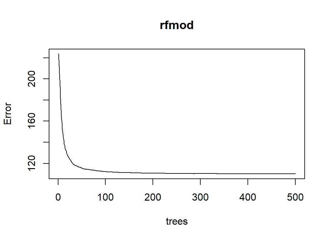
or the values can be extracted from rfmod and plotyed using ggplot.
tibble( trees = 1:500,
        rmse  = sqrt(rfmod$mse)) %>%
  ggplot( aes(x=trees, y=rmse)) +
  geom_line() +
  labs(X="Number of trees", title="Default random forest")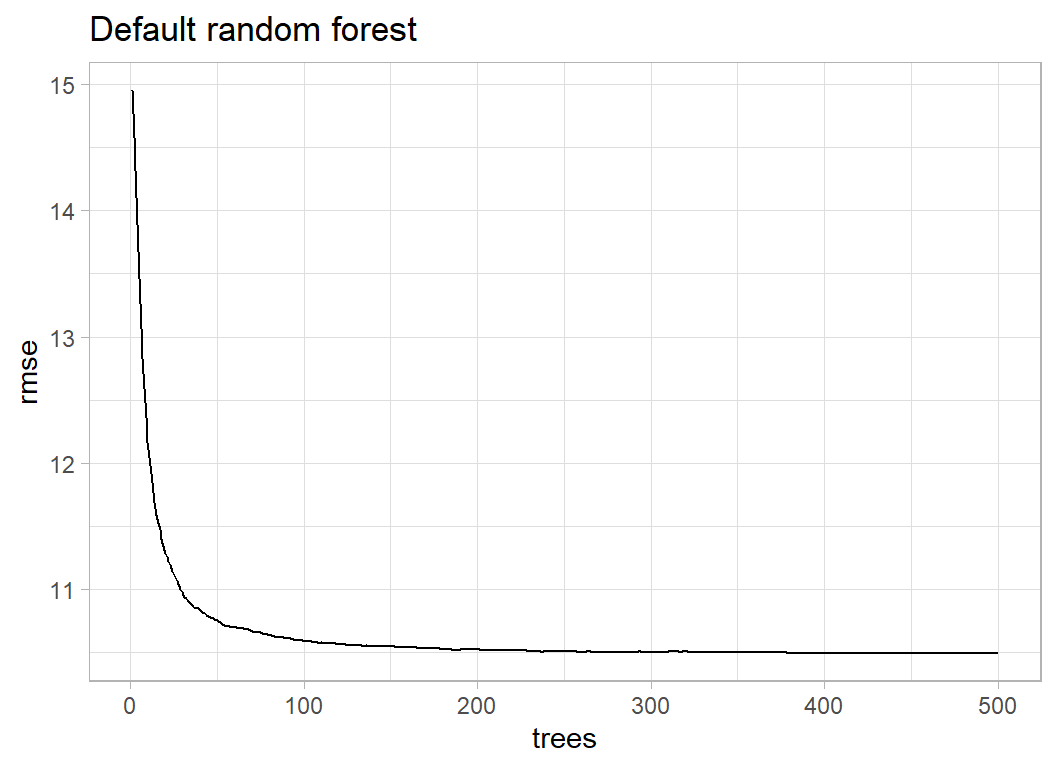
The plot shows that the RMSE drops just below 10.5
For completeness we can look at performance of the model on the validation data
trainDF %>%
   slice(split) %>%
   mutate( yhat = predict(rfmod, newdata=XV)  ) %>%
   summarise( rmse = sqrt( mean( (popularity-yhat)^2 )))
## # A tibble: 1 x 1
## rmse
## <dbl>
## 1 10.7A RMSE of 10.7 is not quite as good and would only just put us in the top ten on the leaderboard.
It is interesting to see which predictors are most important for the model and again we can either use the provided function importance() or we can extract the data and list it for ourselves
# --- extract importance ----------------------------------
tibble( term = attr(rfmod$importance, "dimnames")[[1]],
        purity = as.numeric(rfmod$importance) ) %>%
  mutate( pct = round(100*purity/sum(purity),1) ) %>%
  arrange( desc(purity) ) %>%
  print( n=20)
## # A tibble: 164 x 3
## term purity pct
## <chr> <dbl> <dbl>
## 1 release_year 1249184. 28.7
## 2 avgArtistPop 765214. 17.6
## 3 avgFollowers 445780. 10.2
## 4 acousticness 269354. 6.2
## 5 loudness 195299. 4.5
## 6 duration 128152. 2.9
## 7 energy 123587. 2.8
## 8 danceability 109795. 2.5
## 9 instrumentalness 102694. 2.4
## 10 valence 102378. 2.4
## 11 liveness 99038. 2.3
## 12 speechiness 96683. 2.2
## 13 tempo 88127. 2
## 14 M4 34505. 0.8
## 15 X1 34069. 0.8
## 16 X36 30866. 0.7
## 17 X31 29086. 0.7
## 18 X3 19503. 0.4
## 19 X2 14045. 0.3
## 20 X63 13407. 0.3
## # ... with 144 more rowsI add the percentage of the total purity in order to make it easier to compare the relate importances.
Clearly the release year and the artists popularity are key, followed by the continuous predictors, M4 is the final month of data collection when the popularity had not yet stabilised and the X’s are the key genres.
# --- most important genres -------------------------------
wordsDF %>%
  slice( 1, 36, 31, 3, 2, 63)
## # A tibble: 6 x 5
## term count p_value mWithout mWith
## <chr> <int> <dbl> <dbl> <dbl>
## 1 'classical' 656 4.84e-151 28.2 9.75
## 2 'progressive house' 155 1.37e- 38 27.7 9.22
## 3 'trance' 152 9.09e- 41 27.7 8.98
## 4 'pop' 378 3.87e- 93 27.1 54.6
## 5 'rock' 1143 4.16e-108 27.0 37.6
## 6 'adult standards' 985 1.83e- 23 27.8 22.4I now have the tricky problem of whether or not to try an tune this model. Would different hyperparameters improve performance significantly? The plot of RMSE vs number of trees suggests that the line has plateaued. There is no suggestion that more trees would cause the RMSE to reduce. nodesize is already small, making it larger would only increase the bias. The only option would be to try other values of mtry. Currently, mtry=54, I could perhaps try 44 and 64, but at 10 minutes per run I do not think that this makes much sense.
I am going to settle for this model.
Submission
First the test data have to be preprocessed
testRawDF %>%
  # --- remove extra characters from artist id -------------------
  mutate( id_artists = str_replace_all(id_artists, "\\'", "")) %>%
  mutate( id_artists = str_replace_all(id_artists, "\\[", "")) %>%
  mutate( id_artists = str_replace_all(id_artists, "\\]", "")) %>%
  # --- extract first two artists --------------------------------
  separate(id_artists, into=c("artistId1", "artistId2"), sep=",",
           extra="drop") %>%
  # --- merge first artist ---------------------------------------
  mutate( id_artists = artistId1 ) %>%
     left_join(artistRawDF %>%
                  rename( id_artists = id,
                          follow1    = followers,
                          popArtist1 = popularity) %>%
                  select(id_artists, genres, popArtist1, follow1),
               by = "id_artists")  %>%
  rename( genre1 = genres ) %>%
  mutate( genre1 = ifelse( is.na(genre1), "", genre1 )) %>%
  # --- merge second artist --------------------------------------
  mutate( id_artists = artistId2 ) %>%
  left_join(artistRawDF %>%
               rename( id_artists = id,
                       follow2    = followers,
                       popArtist2 = popularity) %>%
               select(id_artists, genres, popArtist2, follow2),
            by = "id_artists") %>%
  rename( genre2 = genres ) %>%
  mutate( genre2 = ifelse( is.na(genre2), "", genre2 )) %>%
  # --- combine the genres ---------------------------------------
  unite( genre, genre1, genre2,  sep="," ) %>%
  # --- average popularity & followers ---------------------------
  rowwise() %>%
  mutate( avgArtistPop = mean(c(popArtist1, popArtist2),
                              na.rm=TRUE) ) %>%
  mutate( avgFollowers = mean(c(follow1, follow2),
                              na.rm=TRUE) ) %>%
  mutate( avgArtistPop = ifelse( is.nan(avgArtistPop),
                                 NA, avgArtistPop),
          avgFollowers = ifelse( is.nan(avgFollowers),
                                 NA, avgFollowers)) %>%
  # --- drop working variables -----------------------------------
  ungroup() %>%
  select( -artistId1, -artistId2, -popArtist1, -popArtist2,
          -follow1, -follow2, -id_artists)  -> prep1DF

# --- indicators for the top genres -------------------------------
prep1DF <- add_indicators(prep1DF, "genre", wordsDF$term, "X")

# --- indicators for the keys -------------------------------------
prep1DF <- add_indicators(prep1DF, "key", as.character(1:11), "K")

prep1DF %>%
  mutate( artistNA = as.numeric( is.na(avgArtistPop)),
          avgArtistPop = ifelse(is.na(avgArtistPop), 6, avgArtistPop ),
          avgFollowers = ifelse(is.na(avgFollowers), 0, avgFollowers ))  -> prep1DF

prep1DF$name <- ifelse( is.na(prep1DF$name), "", prep1DF$name)
prep1DF <- add_indicators(prep1DF, "name", myWords, "N")

prep1DF$duration <- log10(prep1DF$duration_ms/1000)
prep1DF$release_month <- ifelse( is.na(prep1DF$release_month), 0, prep1DF$release_month)
for( i in 1:4) {
  prep1DF[ paste("M", i, sep="") ] <- as.numeric(prep1DF$release_month == i & prep1DF$release_year == 2021 )
}
saveRDS(prep1DF, file.path(home, "data/rData/processed_test.rds"))
Now we can fit the model to the entire training set and create a submission
trainDF %>%
  pull(popularity) -> Y

trainDF %>%
  select( duration, danceability, energy, loudness, speechiness,
  acousticness, liveness, valence, tempo, instrumentalness,
  avgArtistPop, avgFollowers, release_year, artistNA, M1, M2, M3, M4,
  starts_with("X", ignore.case=FALSE),
  starts_with("N", ignore.case=FALSE),
  starts_with("K", ignore.case=FALSE))  %>%
  as.matrix() -> X

set.seed(1123)
randomForest(x=X, y=Y) %>%
   saveRDS(file.path(home, "data/dataStore/rf_submission1.rds"))
I use this model to create the submission
# --- test sample predictors -----------------------------------
readRDS(file.path(home, "data/rData/processed_test.rds")) %>%
  select( duration, danceability, energy, loudness, speechiness,
  acousticness, liveness, valence, tempo, instrumentalness,
  avgArtistPop, avgFollowers, release_year, artistNA, M1, M2, M3, M4,
  starts_with("X", ignore.case=FALSE),
  starts_with("N", ignore.case=FALSE),
  starts_with("K", ignore.case=FALSE))  %>%
  as.matrix() -> XT

# --- prepare submission --------------------------------------
readRDS(file.path(home, "data/rData/processed_test.rds")) %>%
  mutate( popularity = predict(rfmod, newdata=XT) ) %>%
  select( id, popularity) %>%
  write_csv( file.path(home, "temp/submission1.csv"))
The RMSE of the submission is 10.57712, which would place the model in 4th place on the leaderboard. I think that this is quite a good result, given that random forests are generally inferior to boosted trees and I have not tuned the hyperparameters of the random forest.
What we learn from this analaysis
The novelty, as far as Sliced is concerned, lies in the secondary file of information on the artists. This increases the burden of feature selection and data cleaning but eventually leaves a fairly standard regression problem. I chose random forests because I wanted to try them and not because they are especially suited to this problem, which on reflection was not a good idea.
Random forests work reasonably well for these data; with such a large dataset it is not surprising that large regression trees make good predictions. However, they are very slow to compute and I suspect that they offer no real benefits over quicker algorithms such as boosted trees or even flexible regression models.
I think that it would have been better to have included a feature selection step before building the random forest; many of the keywords extracted from the genres were never likely to be important.
My plan is to re-analyse these data in a later post using a Bayesian mixture model and when I do that, I’ll add feature selection. Bayesian models are also slow to fit and Bayesian mixture models are notoriously tricky.