Sliced Episode 4: Rain Tomorrow
Summary:
Background: In episode 4 of the 2021 series of Sliced, the competitors were given two hours in which to analyse a set of data on daily weather patterns in different parts of Australia. The aim was to predict whether or not it will rain the next day.
My approach: I started with the idea that location would be key to a good model and I tried two approaches, one based on average rainfall patterns for the time of year and the other based on a day’s weather predicting the weather on the following day. I used a Bayesian method to estimate the probability of rain in each month in each location. Before using the daily weather records I imputed the missing data using the mice package. I analysed each location separately by setting up a tibble with one row per location and a list column for the model fits.
Result: My model has an interpretable structure and did reasonably well at prediction. The logloss was about 5% worse than the competition leader.
Conclusion: The model could be improved by adding extra explanatory information including the weather records for the morning, the total rainfall and the wind direction. I omitted these as the post was already very long. However, this problem is best suited to a Bayesian hierarchical model.
Introduction
The fourth of the Sliced datasets can be downloaded from https://www.kaggle.com/c/sliced-s01e04-knyna9. The data describe daily weather conditions in different parts of Australia. The contestants were asked to predict whether or not it would rain on the following day based on those records. Rain tomorrow is a binary response, so the evaluation is by mean logloss.
My initial thoughts are that Australia is a big place and the factors that determine whether it will rain in Darwin might be very different the factors that are predictive in Hobart. Either the model should consider locations separately, or it will need a lot of interactions.
Reading the data
It is my practice to read the data asis and to immediately save it in rds format within a directory called data/rData. For details of the way that I organise my analyses, you should read my post called Sliced Methods Overview.
# --- setup: libraries & options ------------------------
library(tidyverse)
library(lubridate)

theme_set( theme_light())

# --- set home directory -------------------------------
home <- "C:/Projects/kaggle/sliced/s01-e04"

# --- read downloaded data -----------------------------
trainRawDF <- readRDS( file.path(home, "data/rData/train.rds") )

testRawDF <- readRDS( file.path(home, "data/rData/test.rds") )
Data Exploration
Let’s start by inspecting the training data with skim().
# --- summarise with skimr -------------------------------------
skimr::skim(trainRawDF)
As always I have hidden theskimr output, because of its size. It shows that the dataset is quite large; a total of 34,191 daily records from 49 different locations covering the period between 2/11/2007 and 25/6/2017 and it rained on 22.4% of following days.
The potential number of daily weather records for 49 locations between these dates is
as.numeric(as.Date("25-06-2017", format="%d-%m-%Y") -
   as.Date("2-11-2007", format="%d-%m-%Y") ) * 49
## [1] 172627So the training data represent about 20% of all weather records.
Most of the weather records in the training data are over 90% complete, but about 40% of the cloud reports are missing and measures of sunshine and evaporation are almost completely missing.
Ask a silly question
I also used skimr to look at the test data (again I have hidden the output).
# --- summarise with skimr -------------------------------------
skimr::skim(testRawDF)
14,653 weather records from the same 49 locations covering the period 8-11-2007 to 25-6-2017; about 8% of all possible records for that period.
The periods covered by the training and test data are very similar, so the obvious question is whether or not the next day for the test data is in the training data. Let’s check. An inner join gives the matches present in both data frames.
# --- Is the answer given in the training data? --------------------
testRawDF %>%
  # --- the day for which prediction is required -------------------
  mutate( date = date + 1 ) %>%
  select( date, location ) %>%
  # --- merge with the training data -------------------------------
  inner_join( trainRawDF %>%
                select(date, location, rain_today),
              by=c("date", "location"))
## # A tibble: 3,510 x 3
## date location rain_today
## <date> <chr> <dbl>
## 1 2017-06-19 Newcastle 1
## 2 2009-06-27 SydneyAirport 0
## 3 2012-10-27 BadgerysCreek 0
## 4 2010-08-10 Albany 0
## 5 2016-09-20 Woomera 1
## 6 2015-10-17 Woomera 0
## 7 2011-11-22 Cobar 1
## 8 2016-05-08 Townsville 0
## 9 2011-12-24 Watsonia 0
## 10 2016-12-27 Cobar 0
## # ... with 3,500 more rowsSo there are 3,510 day-location combinations in the test data where the day we need to predict is in the training data. 3,510 is about 24% of the test data, so it looks like the test and training data were chosen at random and the organisers forget to ensure that the test data’s prediction days were not in the training data.
Using this information would be against the spirit of the competition, so I’ll ignore it.
Data exploration
Australia is a big place, with a wide range of climates. Woomera is in the desert, Townsville is tropical and Hobart is temperate. Mixing locations might produce very misleading results.
Let’s take Perth as an example, for no other reason than that I visited that city just before the pandemic stopped all travel. It is a beautiful city and must be a great place to live once you get over the remoteness.
# --- rain by month in Perth ---------------------------------
trainRawDF %>%
  filter( location == "Perth" ) %>%
  filter( !is.na(rain_today)) %>%
  mutate( mth = factor(month(date), labels=month.abb)) %>%
  group_by(mth) %>%
  summarise( pctRain = 100*mean(rain_today), .groups="drop") %>%
  ggplot( aes(x=mth, y=pctRain)) +
  geom_bar( stat="identity", fill="steelblue") +
  labs( x = NULL, y= "Percentage of rainy days",
        title="Rainy Days in Perth")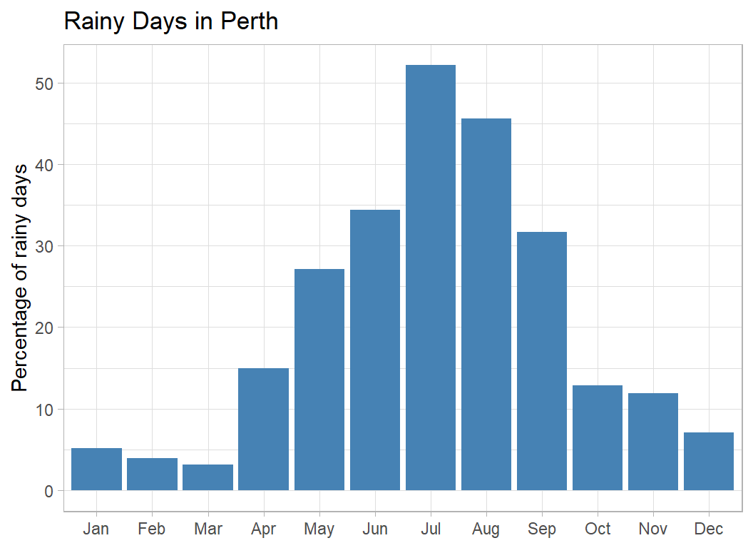
No great surprise that it rains more in the Australian winter, but it is surprising, at least to me, that Perth in July has a higher percentage of rainy days than London in January.
Next let’s look at tropical North Queensland
# --- rain by month in North Queensland ------------------------
trainRawDF %>%
  filter( location == "Townsville" ) %>%
  filter( !is.na(rain_today)) %>%
  mutate( mth = factor(month(date), labels=month.abb)) %>%
  group_by(mth) %>%
  summarise( pctRain = 100*mean(rain_today), .groups="drop") %>%
  ggplot( aes(x=mth, y=pctRain)) +
  geom_bar( stat="identity", fill="steelblue") +
  labs( x = NULL, y= "Percentage of rainy days",
        title="Rainy Days in Townsville")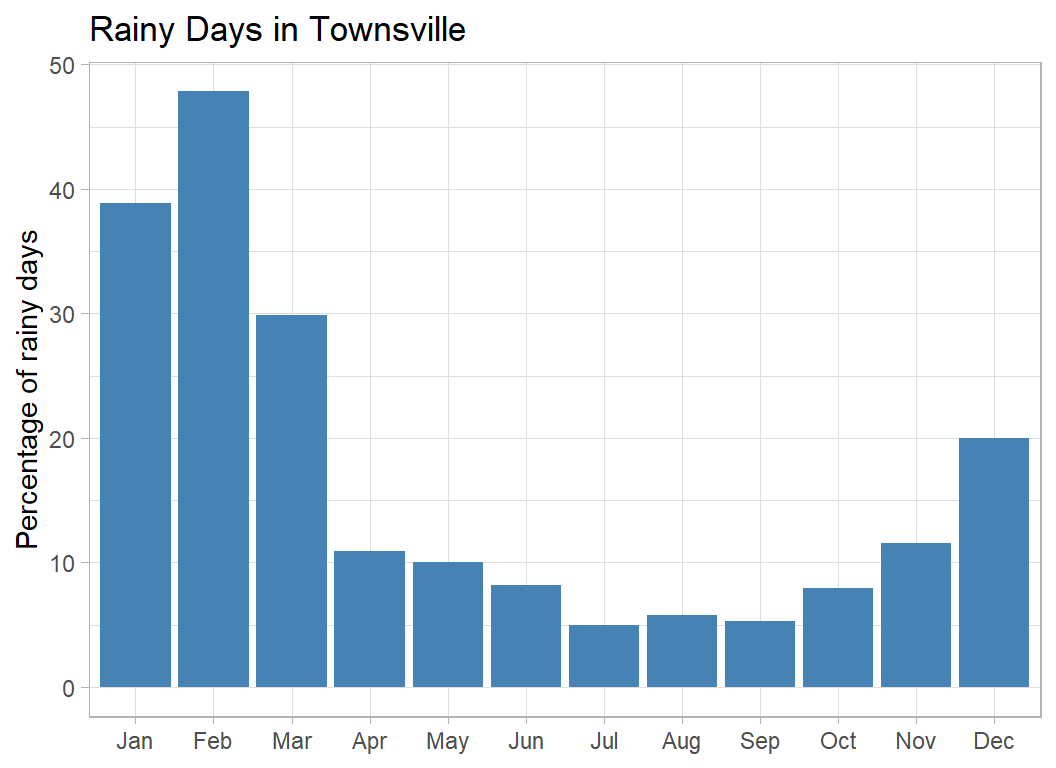
Low rainfall during the Australian winter but high rainfall in the summer months of January and February. Clearly, the Australian average cannot be applied to all locations.
One more example to illustrate a particular problem. I’ve taken the town of Darwin in the Northern Territory. It is like an extreme version of Townsville; wet summers and no rain at all in the winter.
# --- rain by month in Darwin ---------------------------------
trainRawDF %>%
  filter( location == "Darwin" ) %>%
  filter( !is.na(rain_today)) %>%
  mutate( mth = factor(month(date), labels=month.abb)) %>%
  group_by(mth) %>%
  summarise( pctRain = 100*mean(rain_today), .groups="drop") %>%
  ggplot( aes(x=mth, y=pctRain)) +
  geom_bar( stat="identity", fill="steelblue") +
  labs( x = NULL, y= "Percentage of rainy days",
        title="Rainy Days in Darwin")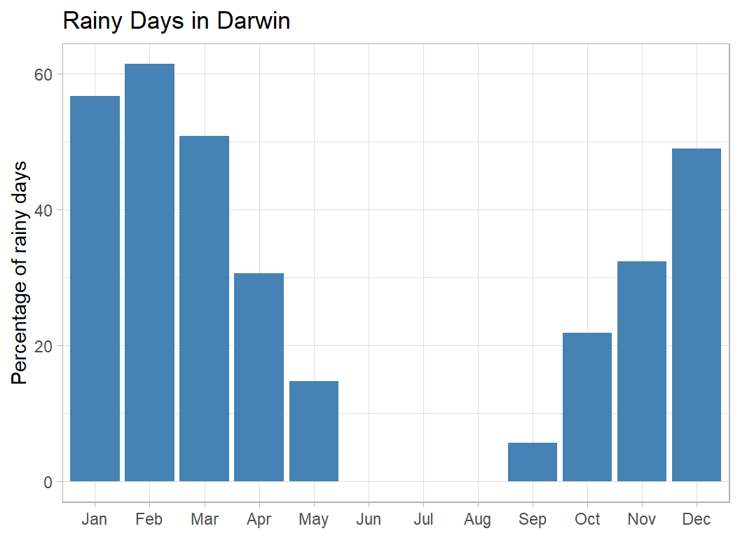
The statistical problem is that there are months when, in this dataset, there were no rainy days. A simple estimate of the probability of rain in June would be zero, i.e. there is a chance of rain on 31st May, but rain on 1st June is impossible. This is counter to common-sense.
A simple model
There are two types of information that we can use to predict rain tomorrow
- long-term averages for that time of the year
- the weather today
My first model will be based on long-term averages. For each location-month combination I will use the percentage of rainy days as the estimate of the probability of rain tomorrow.
trainRawDF %>%
  # --- drop days with missing rain_today ----------------
  filter( !is.na(rain_today)) %>%
  # --- for each location/month combination --------------
  mutate( mth = month(date)) %>%
  group_by(location, mth) %>%
  # --- proportion of rain days --------------------------
  summarise( probRain = mean(rain_today), .groups="drop") %>%
  print() -> probRainDF
## # A tibble: 588 x 3
## location mth probRain
## <chr> <dbl> <dbl>
## 1 Adelaide 1 0.0294
## 2 Adelaide 2 0.0526
## 3 Adelaide 3 0.123
## 4 Adelaide 4 0.193
## 5 Adelaide 5 0.327
## 6 Adelaide 6 0.373
## 7 Adelaide 7 0.415
## 8 Adelaide 8 0.349
## 9 Adelaide 9 0.222
## 10 Adelaide 10 0.254
## # ... with 578 more rowsThe idea is to use these probabilities as the estimates for the test data.
However, as we have already seen, there is a problem. In some places and months, such as Darwin in July, there are no rainy days in the training data, so the estimated probability will be zero. Evaluation is by logloss, which requires the log of the probability estimates; logloss fails when the probability equals 0 or 1. I expect that kaggle has code to cope with zeros, but predictions very close to zero will increase the variance of the metric.
A good way to handle the zeros is with a Bayesian model in which a prior is placed on the monthly probability of rain and the final estimate is a weighted average of the observed probability and the prior probability.
Let’s look at the numbers for Darwin
# --- proportion of rainy days in Darwin ------------------
trainRawDF %>%
  filter( location == "Darwin") %>%
  filter( !is.na(rain_today)) %>%
  mutate( mth = month(date)) %>%
  # --- by month -----------------------
  group_by(mth) %>%
  summarise( n       = n(),
             rainDay = sum(rain_today),
             prop    = rainDay / n,
             .groups = "drop") %>%
  print() %>%
  # --- over the whole year ------------
  ungroup() %>%
  summarise( n       = sum(n),
             rainDay = sum(rainDay),
             prop    = rainDay / n )
## # A tibble: 12 x 4
## mth n rainDay prop
## <dbl> <int> <dbl> <dbl>
## 1 1 74 42 0.568
## 2 2 57 35 0.614
## 3 3 63 32 0.508
## 4 4 49 15 0.306
## 5 5 61 9 0.148
## 6 6 66 0 0
## 7 7 61 0 0
## 8 8 76 0 0
## 9 9 71 4 0.0563
## 10 10 64 14 0.219
## 11 11 68 22 0.324
## 12 12 51 25 0.490## # A tibble: 1 x 3
## n rainDay prop
## <int> <dbl> <dbl>
## 1 761 198 0.260Over the year, 26% of days have rain, but this varies by month from 0% to 61%.
Suppose, in a poor person’s Bayesian analysis, when estimating the probability of rain in a given month, we treat the yearly figure as a crude estimate. So crude that it is only worth 5 days of real data from the month in question. In which case, the yearly proportion of 0.26 would be like observing 1.3 rainy days in 5.
The yearly data can be pooled with the monthly data and get a combined estimate
# --- combination of monthly and annual proportions -----------
trainRawDF %>%
  filter( location == "Darwin") %>%
  filter( !is.na(rain_today)) %>%
  mutate( mth = month(date)) %>%
  group_by(mth) %>%
  summarise( n       = n(),
             rainDay = sum(rain_today),
             prop    = rainDay/n,
             bayes   = (rainDay + 1.3) / (n + 5),
             .groups = "drop" )
## # A tibble: 12 x 5
## mth n rainDay prop bayes
## <dbl> <int> <dbl> <dbl> <dbl>
## 1 1 74 42 0.568 0.548
## 2 2 57 35 0.614 0.585
## 3 3 63 32 0.508 0.490
## 4 4 49 15 0.306 0.302
## 5 5 61 9 0.148 0.156
## 6 6 66 0 0 0.0183
## 7 7 61 0 0 0.0197
## 8 8 76 0 0 0.0160
## 9 9 71 4 0.0563 0.0697
## 10 10 64 14 0.219 0.222
## 11 11 68 22 0.324 0.319
## 12 12 51 25 0.490 0.470The new estimate moves the monthly averages slightly towards the annual estimate. Notice that not all zeros are equal. 0 out of 76 is moved less than 0 out of 61.
Why is the annual figure worth 5 days from a given month? It is subjective. My judgement is that 6 days of data from, say, September tells us slightly more about rain in September than does knowing that Darwin is relatively dry over the year, but, in my judgement, 4 days of data from September is slightly less reliable.
If you feel differently, then in the spirit of Bayes, you should use a different prior.
Let’s build my Bayesian prior into the model
# --- combined estimates for all months & location ----------
trainRawDF %>%
  filter( !is.na(rain_today)) %>%
  mutate( mth = month(date)) %>%
  # --- by month & location ----------------
  group_by(location, mth) %>%
  summarise( n       = n(),
             rainDay = sum(rain_today),
             prop    = rainDay/n,
             .groups="drop") %>%
  # --- annual by location -----------------
  group_by( location) %>%
  mutate( nAnnual    = sum(n),
          rainAnnual = sum(rainDay),
          propAnnual = rainAnnual / nAnnual) %>%
  # --- combined estimates ----------------
  mutate( bayes = (rainDay + propAnnual * 5) / (n + 5) ) %>%
  select( location, mth, prop, bayes) %>%
  print() -> probRainDF
## # A tibble: 588 x 4
## # Groups: location [49]
## location mth prop bayes
## <chr> <dbl> <dbl> <dbl>
## 1 Adelaide 1 0.0294 0.0424
## 2 Adelaide 2 0.0526 0.0660
## 3 Adelaide 3 0.123 0.130
## 4 Adelaide 4 0.193 0.195
## 5 Adelaide 5 0.327 0.318
## 6 Adelaide 6 0.373 0.359
## 7 Adelaide 7 0.415 0.401
## 8 Adelaide 8 0.349 0.340
## 9 Adelaide 9 0.222 0.222
## 10 Adelaide 10 0.254 0.251
## # ... with 578 more rowsThe in-sample logloss for predictions based on these Bayesian estimates is
# --- in-sample logloss -----------------------------
trainRawDF %>%
  mutate( mth = month(date)) %>%
  left_join( probRainDF, by=c("location", "mth")) %>%
  summarise( logloss = -mean( rain_tomorrow*log(bayes) +
                               (1 - rain_tomorrow)*log(1 - bayes)))
## # A tibble: 1 x 1
## logloss
## <dbl>
## 1 0.496Over-fitting should not be a problem because the dataset is large and there has been very little tuning. So the logloss of 0.496 should be a good indicator of performance in the test set.
The sample submission provided by the organisers sets the probability of rain at 0.5 for every location and every day and that base model gets a logloss of 0.693. The best entry on the leaderboard got a logloss of 0.332, which means that my model has some way to go, but let’s be positive, there is a lot of daily weather data that has not yet been used.
Let’s prepare a first submission
testRawDF %>%
  mutate( mth = month(date)) %>%
  select( id, location, mth) %>%
  left_join(probRainDF, by=c("location", "mth")) %>%
  select( id, bayes) %>%
  rename( rain_tomorrow = bayes) %>%
  write.csv(file.path(home, "temp/submission1.csv"),  row.names=FALSE)
This submission had a logloss of 0.502 (based on 99% of the test data). This is very much in line with the in-sample figure of 0.496, but somehow the psychology of going over 0.5 makes it feel worse. Clearly, we will need to make use of the daily weather conditions.
Improved model
We could have got the predictions for our Bayesian model by using a logistic regression. Since a logistic regression models the logit of the probability, I’ll make logitBayes an offset (known term in the model) and I will not have an intercept.
# --- location-month fitted by glm ------------------------
trainRawDF %>%
  mutate( mth = month(date) ) %>%
  left_join( probRainDF, by=c("mth", "location")) %>%
  mutate( logitBayes = log(bayes/(1-bayes)) ) %>%
  glm( rain_tomorrow ~ -1,
         family="binomial", offset=logitBayes, data=.) -> mod

# --- insample logloss ------------------------------------
trainRawDF %>%
  mutate( p = predict(mod, type="response")) %>%
  summarise( logloss = -mean( rain_tomorrow*log(p) +
                               (1 - rain_tomorrow)*log(1 - p)))
## # A tibble: 1 x 1
## logloss
## <dbl>
## 1 0.496The logloss is 0.496, the same as before.
The logistic structure can be used to see if knowing rain_today helps predict rain_tomorrow
library(broom)

# --- long-term average + rain_today -----------------------------
trainRawDF %>%
  filter( !is.na(rain_today)) %>%
  mutate( mth = month(date) ) %>%
  left_join( probRainDF, by=c("mth", "location")) %>%
  mutate( logitBayes = log(bayes/(1-bayes)) ) %>%
  glm( rain_tomorrow ~ rain_today,
         family="binomial", offset=logitBayes, data=.) -> mod

tidy(mod)
## # A tibble: 2 x 5
## term estimate std.error statistic p.value
## <chr> <dbl> <dbl> <dbl> <dbl>
## 1 (Intercept) -0.384 0.0177 -21.7 1.41e-104
## 2 rain_today 1.16 0.0299 38.8 0.rain_today is obviously a very important predictor.
# --- in-sample logloss ------------------------------------
trainRawDF %>%
  filter( !is.na(rain_today)) %>%
  mutate( p = predict(mod, type="response")) %>%
  summarise( logloss = -mean( rain_tomorrow*log(p) +
                               (1 - rain_tomorrow)*log(1 - p)))
## # A tibble: 1 x 1
## logloss
## <dbl>
## 1 0.471A disappointing reduction in in-sample logloss from 0.496 to 0.471, but the comparison is confused by the days on which rain-today is missing.
Let’s look at some of the continuous weather measures. I would imagine that 3pm values are more informative that 9am measures, because they occur closer in time to tomorrow. So I’ll concentrate on 3pm.
Let’s add these factors into the model.
# --- model adding continuous afternoon measures -------------
trainRawDF %>%
  filter( !is.na(rain_today) & !is.na(humidity3pm) &
          !is.na(pressure3pm) & !is.na(temp3pm) &
          !is.na(wind_gust_speed) & !is.na(wind_speed3pm)) %>%
  mutate( mth = month(date) ) %>%
  left_join( probRainDF, by=c("mth", "location")) %>%
  mutate( logitBayes = log(bayes/(1-bayes)) ) %>%
  { glm( rain_tomorrow ~ rain_today + humidity3pm +
           temp3pm + pressure3pm + wind_speed3pm + wind_gust_speed,
         family="binomial", offset=logitBayes, data=.)} -> mod

# --- coefficients -------------------------------------------
tidy(mod)
## # A tibble: 7 x 5
## term estimate std.error statistic p.value
## <chr> <dbl> <dbl> <dbl> <dbl>
## 1 (Intercept) 77.3 3.16 24.5 4.43e-132
## 2 rain_today 0.278 0.0398 6.97 3.21e- 12
## 3 humidity3pm 0.0600 0.00125 48.1 0.
## 4 temp3pm -0.00357 0.00345 -1.04 3.01e- 1
## 5 pressure3pm -0.0812 0.00306 -26.5 6.85e-155
## 6 wind_speed3pm -0.0475 0.00279 -17.0 4.80e- 65
## 7 wind_gust_speed 0.0573 0.00195 29.4 2.33e-190Humidity, pressure and wind speed are clearly important but temperature tells you nothing. We get a similar story from the analysis of deviance table, except that this table is sequential, that is when temperature enters the model we do not yet know about the pressure or the wind-speed, hence it seems more important.
anova(mod)## Analysis of Deviance Table
##
## Model: binomial, link: logit
##
## Response: rain_tomorrow
##
## Terms added sequentially (first to last)
##
##
## Df Deviance Resid. Df Resid. Dev
## NULL 28799 28185
## rain_today 1 1268.91 28798 26916
## humidity3pm 1 2957.15 28797 23959
## temp3pm 1 74.62 28796 23885
## pressure3pm 1 1790.60 28795 22094
## wind_speed3pm 1 16.10 28794 22078
## wind_gust_speed 1 912.67 28793 21165We can look at the distribution of afternoon humidity, when it did or did not rain on the following day.
# --- humidity in the afternoon ------------------------------
trainRawDF %>%
  mutate( rain_tomorrow = factor(rain_tomorrow,
                                 labels=c("no", "yes"))) %>%
  ggplot( aes(x=humidity3pm, fill=rain_tomorrow) ) +
  geom_density( alpha=0.5) +
  labs( title="Humidity at 3pm", fill="rain tomorrow") +
  theme( legend.position = c(0.15, 0.85))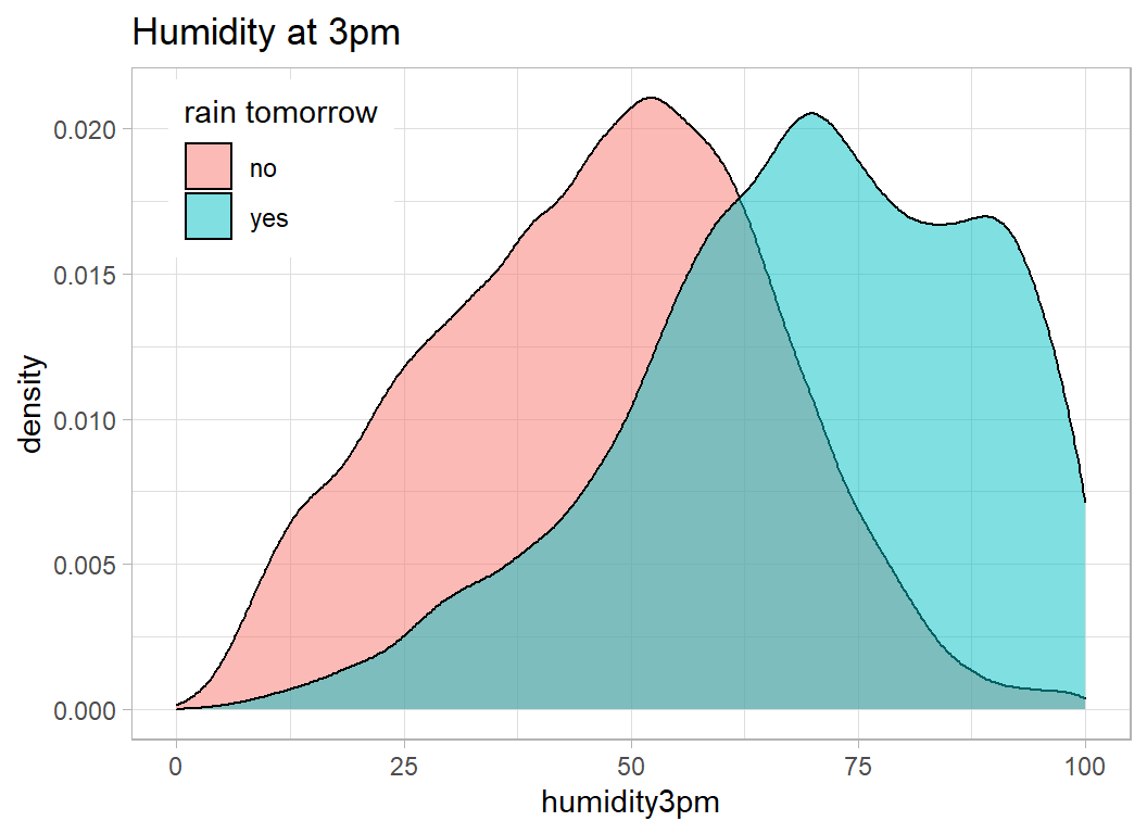
As you would expect high humidity means that rain is more likely (the regression coefficient was positive)
Here is a similar plot for pressure
# --- pressure in the afternoon ------------------------------
trainRawDF %>%
  mutate( rain_tomorrow = factor(rain_tomorrow, labels=c("no", "yes"))) %>%
  ggplot( aes(x=pressure3pm, fill=rain_tomorrow) ) +
  geom_density( alpha=0.5) +
  labs( title="Pressure at 3pm", fill="rain tomorrow") +
  theme( legend.position = c(0.15, 0.85))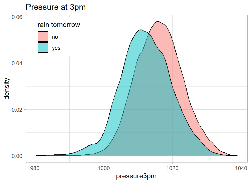
The lower the pressure (negative coefficient), the more likely it is to rain tomorrow, but pressure is less informative than humidity.
What do these extra measurements do to the logloss?
# --- in-sample logloss --------------------------------------
trainRawDF %>%
  filter( !is.na(rain_today) & !is.na(humidity3pm) &
          !is.na(pressure3pm) & !is.na(temp3pm) &
          !is.na(wind_gust_speed) & !is.na(wind_speed3pm) ) %>%
  mutate( p = predict(mod, type="response")) %>%
  summarise( logloss = -mean( rain_tomorrow*log(p) +
                               (1 - rain_tomorrow)*log(1 - p)))
## # A tibble: 1 x 1
## logloss
## <dbl>
## 1 0.367These variables reduce the in-sample logloss from 0.460 to 0.367. At least we are approaching respectability.
In fact, we could calculate the logloss directly from the analysis of deviance table. For a logistic regession model the total logloss is half the residual deviance i.e. 21165/2 = 10582.5 and since there are 28800 observations once we have dropped the missing values, the mean logloss is 10582.5/28800=0.367
So far we have not used cloud cover, an integer measure that ranges from 0 (clear sky) to 8(total cloud cover).
# --- rain tomorrow by cloud cover --------------------------
trainRawDF %>%
  mutate( rain_tomorrow = factor(rain_tomorrow, labels=c("no", "yes"))) %>%
  ggplot( aes(x=cloud3pm, fill=rain_tomorrow) ) +
  geom_bar( position="dodge2") +
  labs( title="Cloud cover at 3pm", fill="rain tomorrow") +
scale_x_continuous( breaks=0:8, limits=c(-0.5, 8.5)) 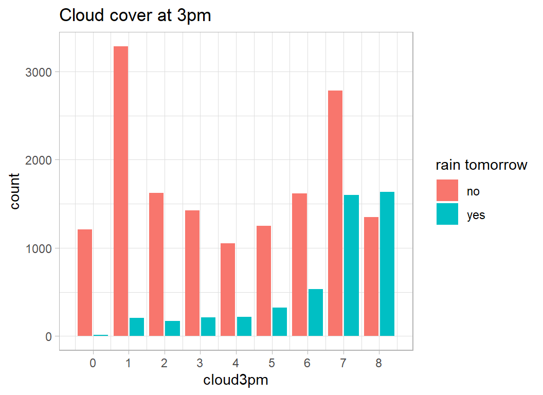
Cloud cover looks to be predictive, but it is frequently missing. Even without cloud cover we lost 15% of the observations due to missing data, add in cloud cover and it will go over 50%. We are going to need imputation.
Imputation
Not only would imputation enable us to use the cloud cover data, but some imputation will be necessary if we are to make predictions for all of the records in the test data using the logistic regression model.
I have decided to use chained regression imputation with the package mice. Briefly, the package sets up a series of regression equations, one for each variable that has missing data. Initial guesses are inserted for the missing values and then the regression equations are fitted to the data and used to improve the guesses. The process is iterated until the predicted missing values stabilise. The imputed values that are taken from the regression equations are selected at random, so that they reflect not only the mean prediction, but also the uncertainty. In this way, mice can be used to create multiple imputations.
Since we will need to impute both the training data and the test data and we want the two imputations to be consistent, I will combine the two data sets and impute on the combined data. I’ll add the percent rainy days by month and location, as I suspect that this might be a good predictor of the missing data.
Wind direction may well be important but it will be difficult to predict. In coastal locations rain is usually associated with wind blowing in from the ocean, but the sea is to the west of Perth, to the east of Sydney and to the south of Adelaide. Imputation by regression equation would be difficult.
# --- combine test and training data ----------------------------
bind_rows(trainRawDF, testRawDF) %>%
  mutate( mth = month(date),
          yr  = year(date))  %>%
  # --- add percent rainy days to fullDF --------------
  left_join(probRainDF,
            by = c("location", "mth")) %>%
  mutate( logitBayes = log(bayes/(1-bayes)) ) %>%
  # make factors --------------------------------------
  select( -evaporation, -sunshine, -prop, -bayes, -date,
          -wind_dir9am, -wind_dir3pm, -wind_gust_dir) %>%
  mutate( rain_today    = factor(rain_today),
          rain_tomorrow = factor(rain_tomorrow),
          location      = factor(location),
          mth           = factor(mth),
          yr            = factor(yr))      -> fullDF
To start with, I will run the default mice imputation with no iterations. This has the effect of getting mice to prepare the imputation without actually running it.
library(mice)

# -- setup chained equations without running them ---------------
imp <- mice(fullDF, maxit=0)

# --- inspect the chosen methods --------------------------------
imp$method
## id location min_temp max_temp rainfall
## "" "" "pmm" "pmm" "pmm"
## wind_gust_speed wind_speed9am wind_speed3pm humidity9am humidity3pm
## "pmm" "pmm" "pmm" "pmm" "pmm"
## pressure9am pressure3pm cloud9am cloud3pm temp9am
## "pmm" "pmm" "pmm" "pmm" "pmm"
## temp3pm rain_today rain_tomorrow mth yr
## "pmm" "logreg" "logreg" "" ""
## logitBayes
## ""In most cases mice recommends pmm (predictive mean matching). This method takes the fitted value of a regression equation for each missing value and then looks for observations with complete data that have similar fitted values. From those cases, one is chosen at random and the actual observation of the selected case is used for imputation. This gives us a random value from the observed uncertainty and saves us from making distributional assumptions.
rain_today and rain_tomorrow are both 0/1 factors and will be modelled by logistic regression. Variables without missing values have no imputation equation and are shown as "".
We are free to change the imputation methods if we wish, but the choices are sensible and you would need good grounds to interfere.
Two issues that needs some thought are the inclusion of rain_tomorrow in the imputation and the use of a single model for all of Australia. rain_tomorrow is the very thing that we are trying to model and it is missing for the test data. So the imputation will give us a prediction for rain_tomorrow in the test set, but it will be an imputed 0/1 value not a probability. The argument for including it, is that rain_tomorrow could be a useful variable when we are trying to impute some of the other missing data, such as missing values of rain_today. Using a single model for all Australia is a practical compromise; given time and effort we could probably do better.
The next thing to inspect is the list of variables that will be used in the regression equations to make the predictions. This structure is stored in a predictor matrix, which is large, so we will look at one line; I’ve chosen the predictors of temp9am.
imp$predictorMatrix["temp9am", ]## id location min_temp max_temp rainfall
## 1 1 1 1 1
## wind_gust_speed wind_speed9am wind_speed3pm humidity9am humidity3pm
## 1 1 1 1 1
## pressure9am pressure3pm cloud9am cloud3pm temp9am
## 1 1 1 1 0
## temp3pm rain_today rain_tomorrow mth yr
## 1 1 1 1 1
## logitBayes
## 1Do we really want to predict temp9am from the id number? Since we do not know how the observations were numbered this would not be advisable. So let’s remove id from all of the prediction equations.
# --- save the methods -------------------------------------
pmeth <- imp$method
# --- don't use id as a predictors -------------------------
pmat <- imp$predictorMatrix
pmat[, c("id")] <- 0
pmat["temp9am", ]
## id location min_temp max_temp rainfall
## 0 1 1 1 1
## wind_gust_speed wind_speed9am wind_speed3pm humidity9am humidity3pm
## 1 1 1 1 1
## pressure9am pressure3pm cloud9am cloud3pm temp9am
## 1 1 1 1 0
## temp3pm rain_today rain_tomorrow mth yr
## 1 1 1 1 1
## logitBayes
## 1Now we can run the imputation. I’ve chosen to run 10 iterations so as to give the imputations time to settle down, the default is 5. It takes a while, so time for a tea break.
# --- create 5 imputed datasets ----------------------------
# --- (10 iterations of the algorithm for each) ------------
set.seed(6728)
mice(fullDF, m = 5, maxit = 10,
             predictorMatrix = pmat,
             method = pmeth, print = FALSE) %>%
saveRDS( file.path(home, "data/rData/imp2.rds") )
Predictions for each location
It is clear that the weather is heavily dependent on location and if we were to model all of the data at the same time, we would need to include a lot of interactions between location and the other measures.
The alternative, which I will adopt, is to have separate models for each location.
When we have developed a prediction model, we will fit it to each of the 5 imputed datasets and then average the predictions of rain tomorrow.
My feeling is that the imputation will induce a degree of over-fitting and so I’ll create a validation set to give us a better idea of model performance than we would get from the in-sample measure.
To start with everything is run on imputed dataset 1. When that is working, I will include the other four imputed datasets.
# --- create estimation and validation sets ---------------------
set.seed(8231)
split <- sample(1:34191, size=10000, replace=FALSE)
# --- extract the first imputation of training data -------------
complete(imp2, action=1) %>%
  slice( 1:34191 ) %>%
  as_tibble() -> trainDF

estimateDF <- trainDF[-split, ]
validateDF <- trainDF[ split, ]
I’ll set up the full analysis in stages, starting with imputation 1 for Perth.
# --- Model for Perth ---------------------------------------------
#

# --- fit prediction model to imputed training data ----------------
estimateDF %>%
  filter( location == "Perth" ) %>%
  { glm( rain_tomorrow ~ rain_today + humidity3pm +
           temp3pm + pressure3pm + wind_speed3pm + wind_gust_speed,
           family="binomial", offset=logitBayes, data=.)} -> mod

# --- coefficients ------------------------------------------------
tidy(mod)
## # A tibble: 7 x 5
## term estimate std.error statistic p.value
## <chr> <dbl> <dbl> <dbl> <dbl>
## 1 (Intercept) 293. 44.1 6.64 3.22e-11
## 2 rain_today1 -0.322 0.356 -0.903 3.66e- 1
## 3 humidity3pm 0.0587 0.0144 4.08 4.41e- 5
## 4 temp3pm -0.218 0.0633 -3.45 5.68e- 4
## 5 pressure3pm -0.287 0.0421 -6.83 8.58e-12
## 6 wind_speed3pm -0.105 0.0428 -2.46 1.40e- 2
## 7 wind_gust_speed 0.0563 0.0235 2.40 1.64e- 2The performance in the validation set
# --- in-sample logloss -------------------------------------------
validateDF %>%
  filter( location == "Perth" ) %>%
  mutate( rain_tomorrow = as.numeric(rain_tomorrow) -1 ) %>%
  mutate( p = predict(mod, type="response", newdata=.)) %>%
  summarise( logloss = -mean( rain_tomorrow*log(p) +
                               (1 - rain_tomorrow)*log(1 - p)))
## # A tibble: 1 x 1
## logloss
## <dbl>
## 1 0.3270.327 is comparable with the top models on the leaderboard, but of course this is just one location and one imputed dataset.
Now that we have set up the method, we can prepare functions that can be used on any chosen location.
# --- modelfit() --------------------------------------------------
# function to fit a model to a selected location
# arguments
#   place  ... name of the chosen location
#   thisDF ... the data frame that we want to analyse
# return
#   fitted model structure
#
modelfit <- function(place, thisDF) {
  thisDF %>%
    filter( location == place) %>%
  { glm( rain_tomorrow ~ rain_today + humidity3pm +
           temp3pm + pressure3pm + wind_speed3pm + wind_gust_speed,
           family="binomial", offset=logitBayes, data=.)} %>%
    return()
}

# --- outsample() --------------------------------------------------
# function to calculate the validation logloss
# arguments
#   place  ... name of the chosen location
#   model  ... fitted model structure
#   thisDF ... the data frame that we want to predict
# return
#   mean logloss
#
outsample <- function(place, model, thisDF) {
  thisDF %>%
    filter( location == place) %>%
    mutate( rain_tomorrow = as.numeric(rain_tomorrow) -1 ) %>%
    mutate( p = predict(model, type="response", newdata=.)) %>%
    summarise( logloss = -mean( rain_tomorrow*log(p) +
                               (1 - rain_tomorrow)*log(1 - p))) %>%
    pull( logloss) %>%
    return()
}

# --- ndays() ----------------------------------------------------
# find number of days of data
# arguments
#   place  ... name of the chosen location
#   thisDF ... the data frame that we want to analyse
# return
#   number of days of data
#
ndays <- function(place, thisDF) {
  thisDF %>%
    filter( location == place) %>%
    summarise( n = n(),
               r = sum(rain_today == "1"),
               pct = round(100*r/n, 1)) %>%
    return()
}
Now we can use the map functions from purrr to fit the same model to every location and save the results in list columns.
# --- separate models for each location -------------------------
tibble( place = unique(trainDF$location) ) %>%
  mutate( model   = map(place, modelfit, thisDF=estimateDF)) %>%
  mutate( n       = map_df(place, ndays, thisDF=estimateDF)) %>%
  mutate( logloss = map2_dbl(place, model, outsample,
                             thisDF=validateDF)) %>%
  print()  -> modDF
## # A tibble: 49 x 4
## place model n$n $r $pct logloss
## <fct> <list> <int> <int> <dbl> <dbl>
## 1 BadgerysCreek <glm> 475 92 19.4 0.334
## 2 Sale <glm> 536 123 22.9 0.319
## 3 Nhil <glm> 263 40 15.2 0.323
## 4 Townsville <glm> 488 76 15.6 0.302
## 5 Uluru <glm> 254 23 9.1 0.200
## 6 Nuriootpa <glm> 518 97 18.7 0.310
## 7 Albany <glm> 524 140 26.7 0.416
## 8 Watsonia <glm> 490 104 21.2 0.365
## 9 Perth <glm> 534 116 21.7 0.327
## 10 Tuggeranong <glm> 467 87 18.6 0.327
## # ... with 39 more rowsWe can see Perth’s 0.327 confirming that the method is working. If we look at the overall result.
modDF %>%
  summarise( mll = mean(logloss, weight=n$n) )
## # A tibble: 1 x 1
## mll
## <dbl>
## 1 0.352The average logloss of 0.352 would only just get us into the top ten on the leaderboard, where the leading model scored 0.332.
Here are the locations that are poorly predicted.
modDF %>%
  arrange( desc(logloss))
## # A tibble: 49 x 4
## place model n$n $r $pct logloss
## <fct> <list> <int> <int> <dbl> <dbl>
## 1 NorfolkIsland <glm> 527 173 32.8 0.524
## 2 SydneyAirport <glm> 497 123 24.7 0.484
## 3 CoffsHarbour <glm> 454 135 29.7 0.478
## 4 Portland <glm> 510 184 36.1 0.470
## 5 Williamtown <glm> 454 106 23.3 0.464
## 6 Cairns <glm> 529 177 33.5 0.460
## 7 Launceston <glm> 499 118 23.6 0.458
## 8 Melbourne <glm> 381 90 23.6 0.456
## 9 NorahHead <glm> 490 137 28 0.439
## 10 Newcastle <glm> 518 127 24.5 0.434
## # ... with 39 more rowsMy impression is that these locations are relatively rainy. This impression is supported by plotting logloss against percent rainy days for the 49 locations.
# --- logloss vs pct rainy days by location ------------------
modDF %>%
  ggplot( aes(x=n$pct, y=logloss)) +
  geom_point() +
  labs( x = "percent rainy days",
        y = "mean log loss")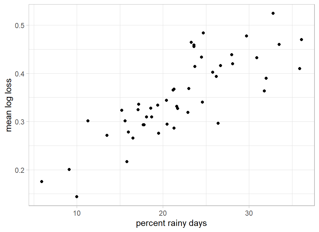
So far we have only looked at imputation 1, so now I’ll loop through all of the imputed datasets.
set.seed(2964)
# --- vector to save the results ----------------------------------------
avgLogLoss <- rep(0, 5)
# --- loop over the 5 imputations ---------------------------------------
for( iset in 1:5 ) {
  # --- extract the required imputed training data ----------------------
  complete(imp2, action=iset) %>%
    slice( 1:34191 ) %>%
    as_tibble() -> trainDF

  split <- sample(1:34191, size=10000, replace=FALSE)
  estimateDF <- trainDF[-split, ]
  validateDF <- trainDF[ split, ]

  # --- calculate the out of sample mean logloss ----------------------
  tibble( place = unique(trainDF$location) ) %>%
     mutate( model   = map(place, modelfit, thisDF=estimateDF)) %>%
     mutate( n       = map_df(place, ndays, thisDF=estimateDF)) %>%
     mutate( logloss = map2_dbl(place, model, outsample,
                                thisDF=validateDF)) %>%
     summarise( mll  = mean(logloss, weight=n$n) ) %>%
     pull(mll) -> avgLogLoss[iset]
}
summary(avgLogLoss)
## Min. 1st Qu. Median Mean 3rd Qu. Max.
## 0.3337 0.3384 0.3395 0.3420 0.3470 0.3514The loglosses across the 5 imputed datasets are very consistent and average 0.342.
Submission
I will fit the model to each imputed training set and then make predictions for the corresponding imputed test set. The submission will be the average of the 5 predicted probabilities.
We will need a function that returns the predictions for a given location.
# --- predict_rain() --------------------------------------------------
# function to predict rain_tomorrow
# arguments
#   place  ... name of the chosen location
#   model  ... fitted model structure
#   thisDF ... data frame with predictors
# return
#   data frame with id and prediction
#
predict_rain <- function(place, model, thisDF) {
  thisDF %>%
    filter( location == place) %>%
    mutate( rain_tomorrow = predict(model,
                                    type="response", newdata=.)) %>%
    select(id, rain_tomorrow) %>%
    return()
}
Test the function on the first imputation
# --- training data for imputation 1 -----------------------
complete(imp2, action=1) %>%
  slice( 1:34191 ) %>%
  as_tibble() -> trainDF

# --- test data for imputation 1 ---------------------------
complete(imp2, action=1) %>%
  slice( 34192:48844 ) %>%
  as_tibble() -> testDF

# --- predicted probabilities ------------------------------
tibble( place = unique(trainDF$location) ) %>%
  mutate( model = map(place, modelfit, thisDF=trainDF)) %>%
  mutate( p     = map2(place, model, predict_rain, thisDF=testDF)) %>%
  select(p) %>%
  unnest(p)
## # A tibble: 14,653 x 2
## id rain_tomorrow
## <dbl> <dbl>
## 1 2036 0.205
## 2 41258 0.00598
## 3 37733 0.0585
## 4 41920 0.0866
## 5 15188 0.111
## 6 7118 0.838
## 7 22425 0.0879
## 8 26516 0.0517
## 9 40344 0.867
## 10 10035 0.0286
## # ... with 14,643 more rowsNow I’ll make predictions for all locations and all 5 imputed datasets
# --- predictions for all 5 imputed datasets --------------------
for( iset in 1:5 ) {
  # --- extract the required imputed training data --------------
  complete(imp2, action=iset) %>%
    slice( 1:34191 ) %>%
    as_tibble() -> trainDF

  complete(imp2, action=iset) %>%
    slice( 34192:48844 ) %>%
    as_tibble() -> testDF

# --- predicted probabilities ------------------------------
  tibble( place = unique(trainDF$location) ) %>%
    mutate( model = map(place, modelfit, thisDF=trainDF)) %>%
    mutate( p     = map2(place, model,
                         predict_rain, thisDF=testDF)) %>%
    select(p) %>%
    unnest(p) %>%
    saveRDS( file.path(home,
              paste("data/rData/pred", iset, ".rds", sep="")) )
}
Let’s combine the saved predictions and see how they vary.
# --- read and combine the predictions --------------------
bind_rows(
   readRDS( file.path(home, "data/rData/pred1.rds")),
   readRDS( file.path(home, "data/rData/pred2.rds")),
   readRDS( file.path(home, "data/rData/pred3.rds")),
   readRDS( file.path(home, "data/rData/pred4.rds")),
   readRDS( file.path(home, "data/rData/pred5.rds")),
          .id="imputation") -> predictionDF
# --- inspect the predictions  ----------------------------
predictionDF %>%
  pivot_wider(values_from=rain_tomorrow, names_from=imputation)
## # A tibble: 14,653 x 6
## id `1` `2` `3` `4` `5`
## <dbl> <dbl> <dbl> <dbl> <dbl> <dbl>
## 1 2036 0.205 0.205 0.194 0.211 0.202
## 2 41258 0.00598 0.00590 0.00580 0.00599 0.00589
## 3 37733 0.0585 0.0541 0.0577 0.0561 0.0552
## 4 41920 0.0866 0.0866 0.0856 0.0869 0.0861
## 5 15188 0.111 0.109 0.112 0.109 0.109
## 6 7118 0.838 0.842 0.838 0.841 0.838
## 7 22425 0.0879 0.0885 0.0848 0.0897 0.0880
## 8 26516 0.0517 0.0528 0.0506 0.0528 0.0526
## 9 40344 0.867 0.865 0.866 0.866 0.864
## 10 10035 0.0286 0.0275 0.0281 0.0281 0.0280
## # ... with 14,643 more rowsThere is broad agreement. Obviously, the predictions will vary more for days that had missing values in key predictors.
The actual submission will be based on the average prediction. There is an argument for averaging on a logit scale, but that seems over the top.
Here is the average prediction across imputations.
# --- create submission from the average prediction -------------------
predictionDF %>%
  group_by(id) %>%
  summarise( rain_tomorrow = mean(rain_tomorrow), .groups="drop") %>%
  select( id, rain_tomorrow) %>%
  print() %>%
  write.csv( file.path(home, "temp/submission2.csv"),
             row.names=FALSE)
## # A tibble: 14,653 x 2
## id rain_tomorrow
## <dbl> <dbl>
## 1 1 0.344
## 2 2 0.253
## 3 3 0.134
## 4 4 0.975
## 5 11 0.303
## 6 12 0.368
## 7 16 0.0785
## 8 21 0.00777
## 9 22 0.100
## 10 24 0.00275
## # ... with 14,643 more rowsWhen I submitted this file the logloss was calculated as 0.35636. The top model scored 0.33173, so my model’s performance is a little disappointing.
What this example shows
This quite a hard example for a two hour competition; days within locations and lots of missing data.
I quite like the idea of the Bayesian estimates of the proportion of days on which it rained calculated by location and month. Given more time, it would be interesting to extend the Bayesian approach and to fit a hierarchical Bayesian model to the full data set. There is an obvious structure of weather features within locations that would be perfectly suited to Bayesian estimation. The impact of, say, humidity on rain tomorrow could be viewed as an average effect for all Australia plus a random effect over locations. This would mean that each location’s regression coefficients would be shrunk towards the Australian average. A big advantage of such a model would be that it could be fitted to the data without the need for imputation.
The use of list columns to store multiple models is described by Hadley Wickham in his on-line book, R for Data Science, at https://r4ds.had.co.nz/many-models.html and in a video at https://www.youtube.com/watch?v=rz3_FDVt9eg. These data provide a nice example of the method, but they also highlight the limitation of analysing one location without taking the others into account. At the least, location ought to be grouped by position within Australia, for instance, Sydney and Newcastle ought to experience similar weather patterns.
The imputation has left me with concerns, chiefly that having stressed the importance of location in modifying the effect of say humidity on rainfall, the imputation model only used average effects.
No doubt the model performance could have been improved by using more of the daily weather data. I left out, the morning records, the total rainfall and the wind direction.
Another weakness, from a machine learning perspective, is the limited data visualisation. My own feeling is that if you use interpretable models, then the models will convey the same messages as the visualisations. Pretty maps might have looked good, but I do not think that they would have added much.
Having had the experience of this analysis, were I to start again I would definitely use stan to fit a Bayesian model. My aim is to analyse all of the Sliced datasets and then to revisit them. I have in mind a post on generalized additive models and splines as a background to episode 1, so perhaps I will write a post on Bayesian analysis linked to these data.