Methods: Nimble HMC (Second thoughts)
Introduction
It is only yesterday that I wrote a post on nimbleHMC and already I have had second thoughts, some positive and some not so positive. In yesterday’s post, I hit a problem with dynamic indexing and I needed a work around based on dummy variables. Shortly, after posting I realised that there was a much simpler solution, which I’ll explain below. However, when I tested my new code, I realised that there were other issues that I had missed.
I wrote this current post as I tried different variations on yesterday’s HMC analysis, so it has ended as a kind of diary rather than a structured explanation. For that reason, it might be easier to follow if you see in advance the conclusions that I reached at the end of the process. Here they are,
- I remain optimistic that HMC will make nimble a more competitive option for Bayesian model fitting
- nimble’s default random walk MCMC is not a great algorithm
- No Monte Carlo algorithm is ever fully automatic
- Entering the explanatory variables as constants rather than data overcomes the dynamic indexing problem.
- The dynamic indexing and the dummy variables parameterisations gave similar results in similar run-times.
- Playing with a beta version of a package is a process of trial and error
- You need to be very careful with Object Orientated Programming (OOP) software, because it is in the nature of OOP that objects can change internally without you realising, which means that a second run of apparently identical code will not necessarily give the same results as a first run. Be careful.
- The long run times that I experienced with some analyses seem to have been due to too short a warm-up leading to a poorly tuned algorithm. It was not a problem of setting up the automatic differentiation (A)D as I initially suspected.
- Given the importance of tuning an algorithm to each specific problem,
nimbleneeds to make it easy for the user to control the algorithm.
Dynamic Indexing
In yesterday’s post, I started by writing my Poisson regression model in this form,
library(nimble)

# --- Model code as used previously ------------------------------
nimbleCode( {
  for( i in 1:560 ) {
    log(mu[i]) <- b0 + b1*year[i] + b2[age[i]] + b3*gender[i] + offset[i]
    deaths[i] ~ dpois(mu[i])
  }
  b0 ~ dnorm(0, 0.0001)
  b1 ~ dnorm(0, 0.0001)
  b2[1] <- 0.0
  for(j in 2:14) {
    b2[j] ~ dnorm(0, 0.0001)
  }
  b3 ~ dnorm(0, 0.0001)
} )                       -> modelCode
Unfortunately, nimble could not cope with the expression b2[age[i]], which caused a problem for the automatic differentiation (AD) needed by the HMC algorithm.
Almost as soon as I had pressed the button to publish the post, I realised that I had entered age as data, as you would in OpenBUGS, while nimble allows both data and constants.
I could have entered the explanatory variables as constants and the response variable as data as shown below.
# --- Explanatory data as constants ------------------------------
nimbleConst <- list(offset = log(alcDF$pop),
                    year   = alcDF$year - 2001,
                    gender = as.numeric( alcDF$gender == "male"),
                    age    = as.numeric(alcDF$age) )

# --- response variable as data ----------------------------------
nimbleData <- list( deaths = alcDF$deaths)

# --- initial values (as before) ---------------------------------
nimbleInits <-
  list( b1=0, b2=c( NA, rep(0,13)), b3=0)
Now the model becomes
# --- create the model ---------------------------------
nimbleModel(
  code      = modelCode,
  data      = nimbleData,
  constants = nimbleConst,
  inits     = nimbleInits,
  buildDerivs = TRUE ) -> model
This compiles without problem, so we can continue as before.
library(nimbleHMC)

# --- Compile the model ---------------------------------
modelCompiled <- compileNimble(model)

# --- select the samplers ---------------------------------
modelHMC <- buildHMC(model)

# --- compile the sampling algorithm ----------------------
hmcCompiled <- compileNimble(modelHMC, project=model)

# --- run the compiled nimble code ----------------------
runMCMC(
  mcmc    = hmcCompiled,
  niter   = 1000,
  setSeed = 1832
)  %>%
  saveRDS( file.path( home, "data/dataStore/testHMC01.rds")) %>%
  system.time()
Running this code I found a huge increase in run-time, what has previously taken well under 10 seconds was now taking 75 seconds.
I thought at first that I might have been running some R code instead of the compiled code, I know that both methods are possible within nimble. Then I discovered that if I re-run the runMCMC() command without any recompilation, the run-time drops from 75 seconds to 9 seconds.
A possible explanation is that when first running the code, nimble needs to work out the details of the algorithm for calculating the derivatives, essentially through a series of applications of the chain rule. Once that algorithm is established, it is repeated and the calculation is relatively quick. This method is not forgotten, so when the chain is rerun, the run-time drops enormously. For this example, it looks as though it takes over a minute to establish the AD algorithm, which seems unrealistically long.
This raises the question of whether it would be quicker if I were to use yesterday’s reparameterisation in terms of dummy age variables.
I decided to run a few tests. I am afraid that those tests were rather quick and dirty in the sense that I ran each configuration only once. Run-times can vary depending on what other software is running in the background on the computer, so do not read too much into a run-time differences of few seconds either way. None the less, it does appear that the big determining factor is between the first run and any subsequent run. Parameterisation or movement of the explanatory variables between the data and the constants made almost no difference.
The trouble with OOP
Deep inside, nimble uses the R6 package to implement Object Orientated Programming (OOP). I am not particularly keen on OOP for one main reason; objects are mutable, that is to say they can change without you being aware of it. This has its uses, but it makes it impossible to trace exactly what has happened when you run code that you did not write.
In this case, nimble seems to remember the state of the chain, so that a second run picks up from where the previous run ended, which could be very useful. The danger here is that when running OOP code, it is easy to become confused whether you are actually running from scratch and this will have an impact on both timing and performance. The fact that yesterday my timing for 1000 iterations was so quick suggests that I had run the same code before without realising it. This means that the convergence of the chain might also be misleading. I need to go back and ensure that everything is run from scratch.
Let’s start again
Just so that we are clear, the code above with age entered as a constant and dynamic indexing takes about 75 seconds to run first time and about 9 seconds to re-run.
Here is a trace plot of the chain for the year coefficient, obtained from the the first run after I had started a fresh R session.
library(MyPackage)

# --- read the result -----------------------------------------
readRDS(file.path( home, "data/dataStore/testHMC01.rds")) %>%
  nimble_to_df() -> simDF

# --- trace plot of b1 -------------------------------
trace_plot(simDF, b1, iter) +
  labs(title="HMC: Year coefficient (median and 80% interval)")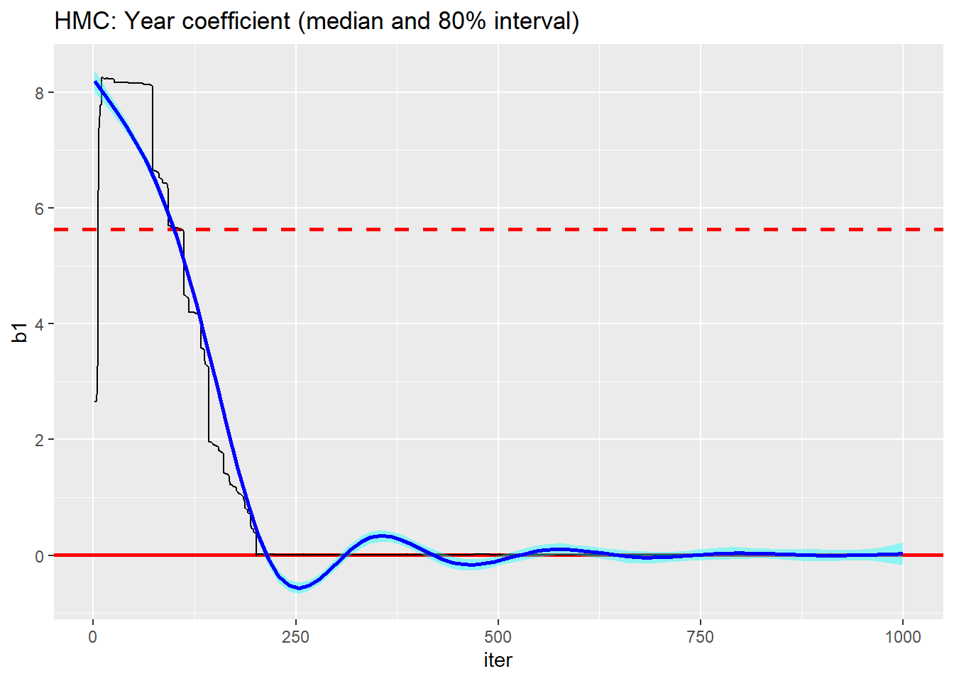
The performance is terrible, nothing like the performance that I got yesterday. Is this due to parameterisation or to inadvertently re-running yesterday’s chain.
I’ll re-run the same code. This takes about 7 seconds.
# --- run the compiled nimble code ----------------------
runMCMC(
  mcmc    = hmcCompiled,
  niter   = 1000,
  setSeed = 1832
)  %>%
  saveRDS( file.path( home, "data/dataStore/testHMC02.rds")) %>%
  system.time()
This is the new trace plot.
# --- read the result -----------------------------------------
readRDS(file.path( home, "data/dataStore/testHMC02.rds")) %>%
  nimble_to_df() -> simDF

# --- trace plot of b1 -------------------------------
trace_plot(simDF, b1, iter) +
  labs(title="HMC: Year coefficient (second run)")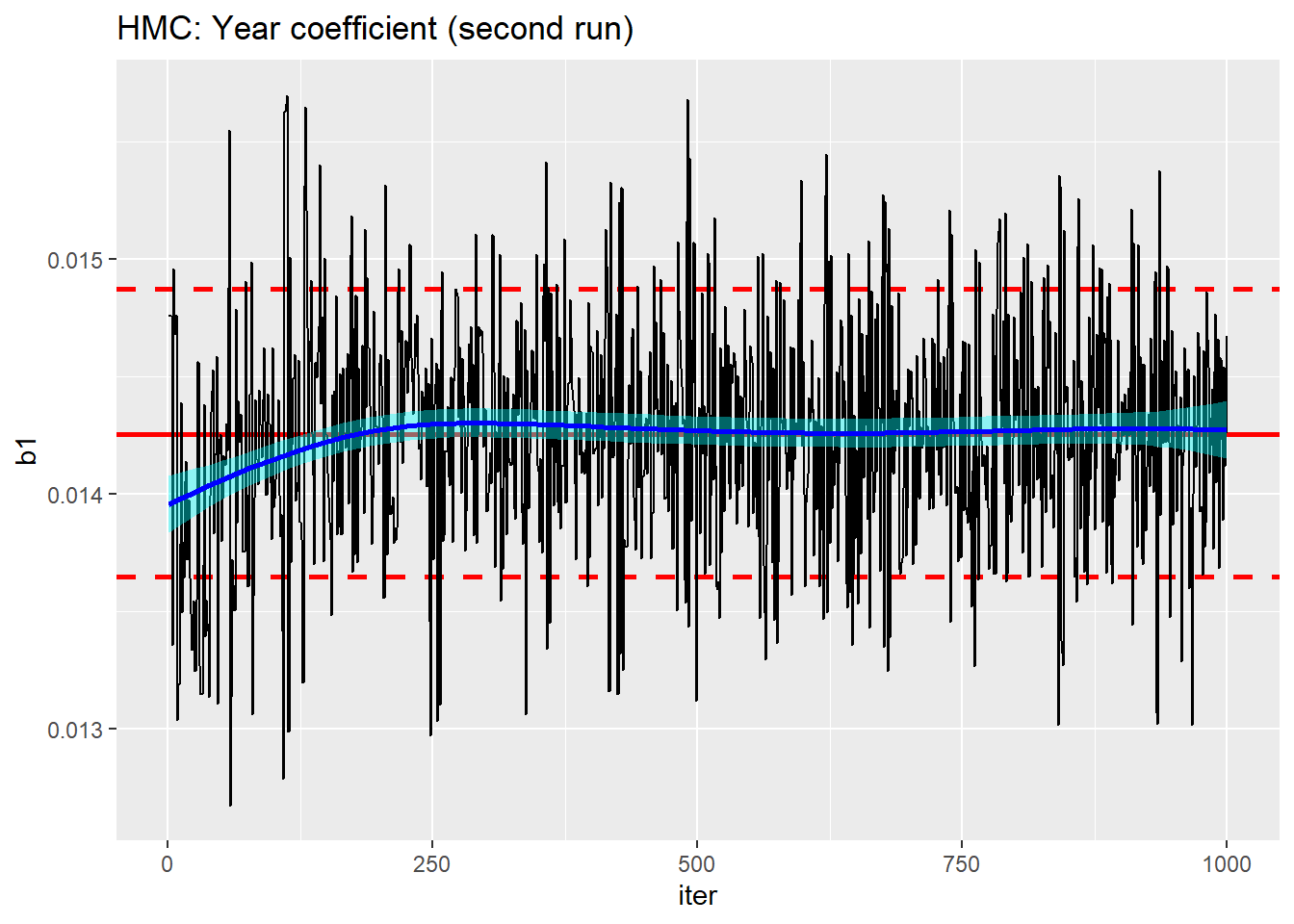
Clearly, nimble has built the second run on what it learnt during the first run.
Here is the trace plot following a third run
# --- read the result -----------------------------------------
readRDS(file.path( home, "data/dataStore/testHMC03.rds")) %>%
  nimble_to_df() -> simDF

# --- trace plot of b1 -------------------------------
trace_plot(simDF, b1, iter) +
  labs(title="HMC: Year coefficient (third run)")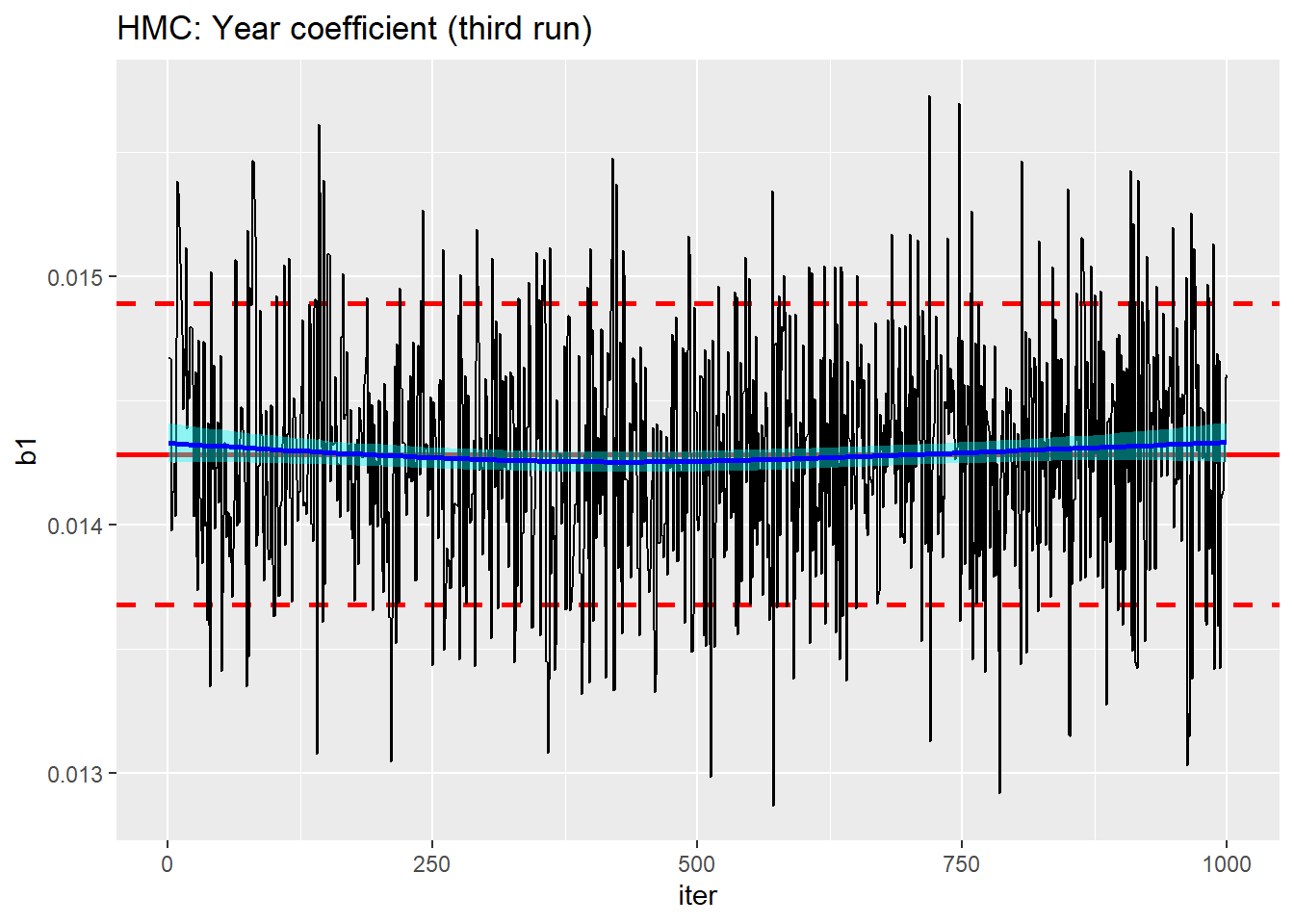
We seem to be close to convergence for b1, but how about the other parameters. Here is a trace plot of the second age term obtained from the third run of the algorithm.
# --- trace plot of b2_2 -------------------------------
trace_plot(simDF, b2_2, iter) +
  labs(title="HMC: Age2 coefficient (third run)")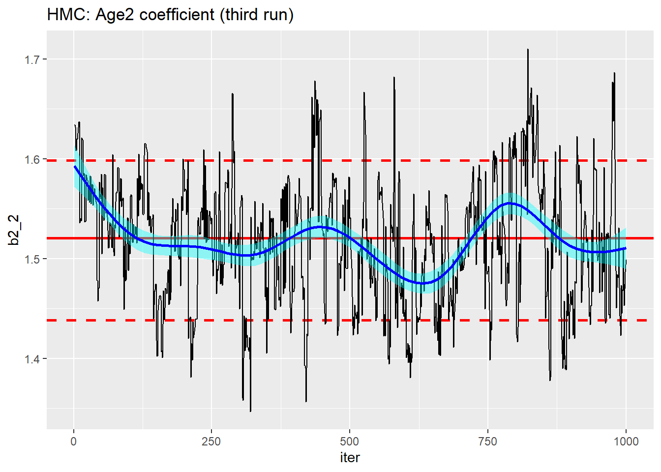
Even on the third run, this still resembles the results of a poor random walk MCMC sampler.
It is not too surprising that the age coefficients are less well estimated. b2_2 is the contrast between age group 2 and the base age and can only be estimated from a fraction of the data, what is more, the coefficient will be correlated with the intercept, making convergence even slower.
Is the poor performance due to the parameterisation? I ran the version with dummy variables in place of dynamic indexes and repeated it three times as above. Here is the result for b2_2
# --- read the result -----------------------------------------
readRDS(file.path( home, "data/dataStore/testHMC04.rds")) %>%
  nimble_to_df() -> simDF

trace_plot(simDF, b2_2, iter) +
  labs(title="HMC: Age2 coefficient (dummy variable parameterisation)")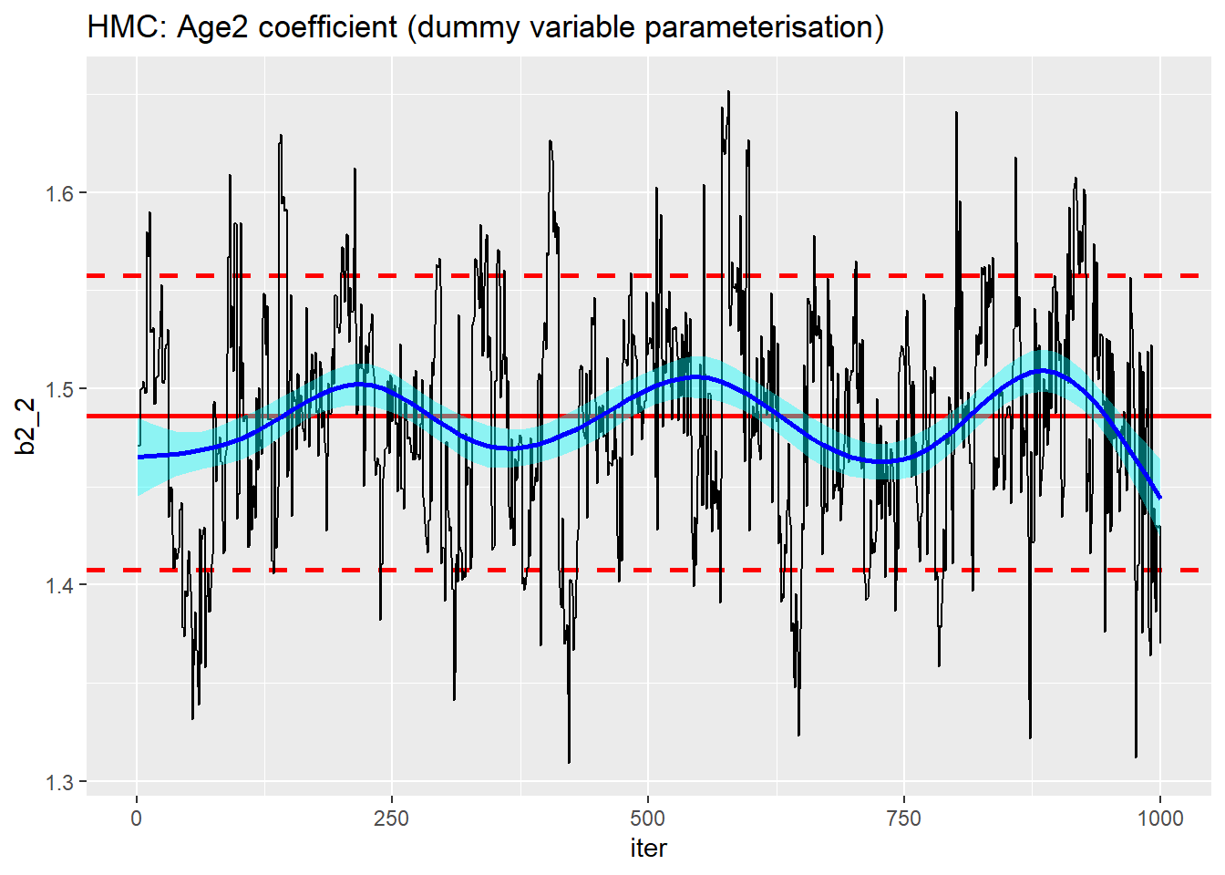
Not much to choose between the parameterisations.
Improving performance
In my limited experience, stan does well not just because it uses HMC, but also because the programmers have put a lot of effort into tuning the algorithm to the needs of each particular problem. This includes the way that they have used the warm-up period to select good control parameters and to make sure that the actual run starts close to the centre of the posterior.
My short runs of 1000 iterations trigger a warm-up of 500 iterations, taken together with my poor initial values this might well be too short.
Let’s try a longer run with better starting values. I’ll base my starting values on the equivalent generalised linear model.
# --- Poisson regression using glm() ------------------------------------------
library(broom)

glm( deaths ~ year + age + gender,
     data   = alcDF %>% mutate( year = year - 2001),
     family = "poisson",
     offset = log(pop)) %>%
  tidy()
## # A tibble: 16 × 5
## term estimate std.error statistic p.value
## <chr> <dbl> <dbl> <dbl> <dbl>
## 1 (Intercept) -1.68 0.0586 -28.7 4.82e-181
## 2 year 0.0143 0.000465 30.7 4.63e-207
## 3 age25-29 1.50 0.0646 23.2 7.12e-119
## 4 age30-34 2.53 0.0606 41.7 0
## 5 age35-39 3.25 0.0594 54.7 0
## 6 age40-44 3.81 0.0590 64.5 0
## 7 age45-49 4.18 0.0588 71.1 0
## 8 age50-54 4.37 0.0587 74.4 0
## 9 age55-59 4.44 0.0587 75.6 0
## 10 age60-64 4.42 0.0588 75.2 0
## 11 age65-69 4.26 0.0589 72.3 0
## 12 age70-74 3.90 0.0593 65.7 0
## 13 age75-79 3.53 0.0602 58.7 0
## 14 age80-84 3.06 0.0624 49.0 0
## 15 age85+ 2.41 0.0671 35.9 1.60e-281
## 16 gendermale 0.778 0.00571 136. 0This suggests better starting values would be
nimbleInits <- list( b0 = -2, b1 = 0,
                     b2 = c( NA, rep(3, 13)), b3 = 1)
Running a 1000 iteration chain from these starting values produces
# --- read the result -----------------------------------------
readRDS(file.path( home, "data/dataStore/testHMC05.rds")) %>%
  nimble_to_df() -> simDF

trace_plot(simDF, b2_2, iter) +
  labs(title="HMC: Age2 coefficient (better starting values)")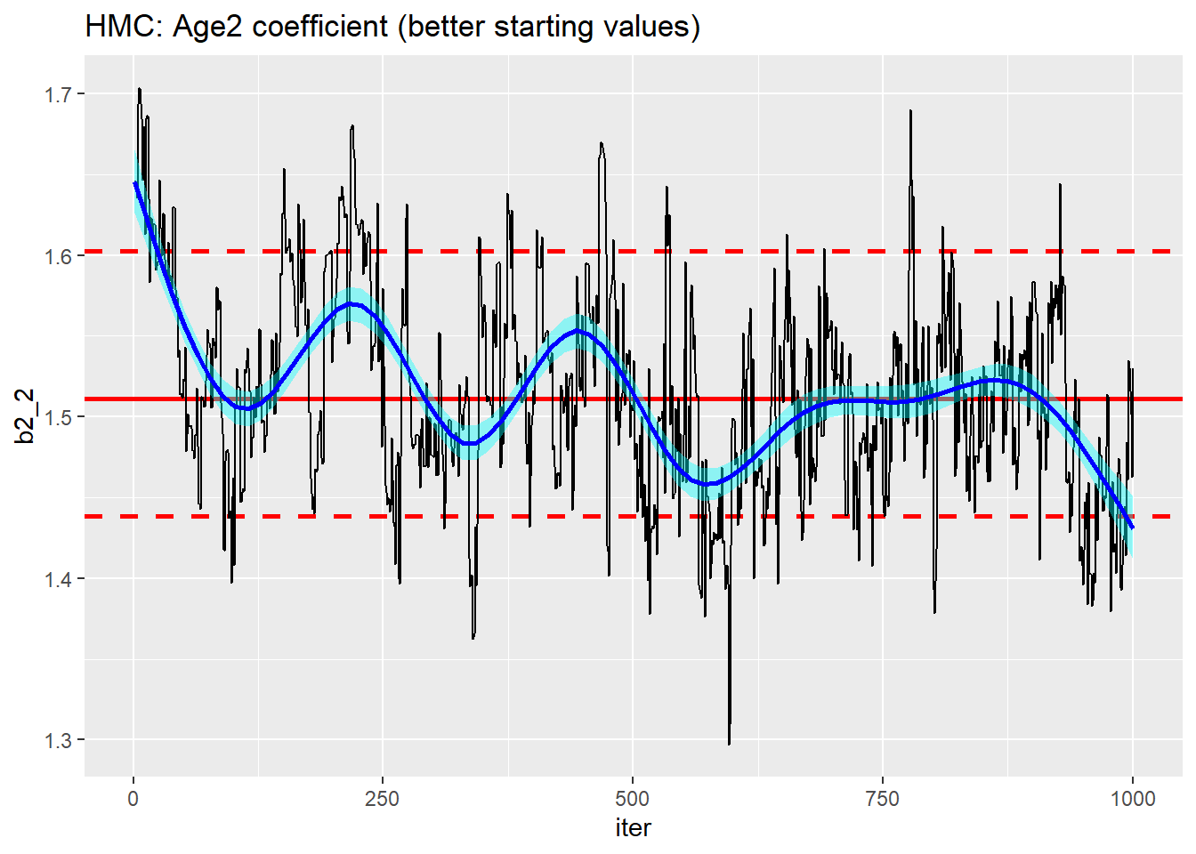
Really no better. The algorithm might have found the centre of the posterior more quickly, but mixing is still poor.
How about a longer warm-up. I cleared everything and then ran from scratch with the better initial values and 3000 iterations. The warm-up jumped from 500 to 1000 iterations.
Here is the performance after a single run of 3000.
# --- read the result -----------------------------------------
readRDS(file.path( home, "data/dataStore/testHMC06.rds")) %>%
  nimble_to_df() -> simDF

trace_plot(simDF, b2_2, iter) +
  labs(title="HMC: Age2 coefficient (3000 iterations)")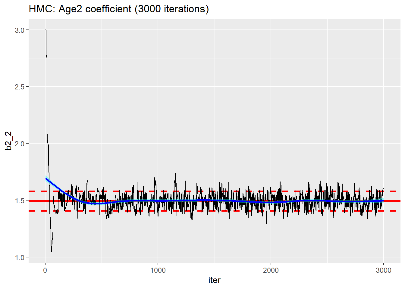
Except for the very start of the chain, the performance looks better
trace_plot(simDF %>% filter(iter > 500), b2_2, iter) +
  labs(title="HMC: Age2 coefficient (discarding the first 500 iterations)")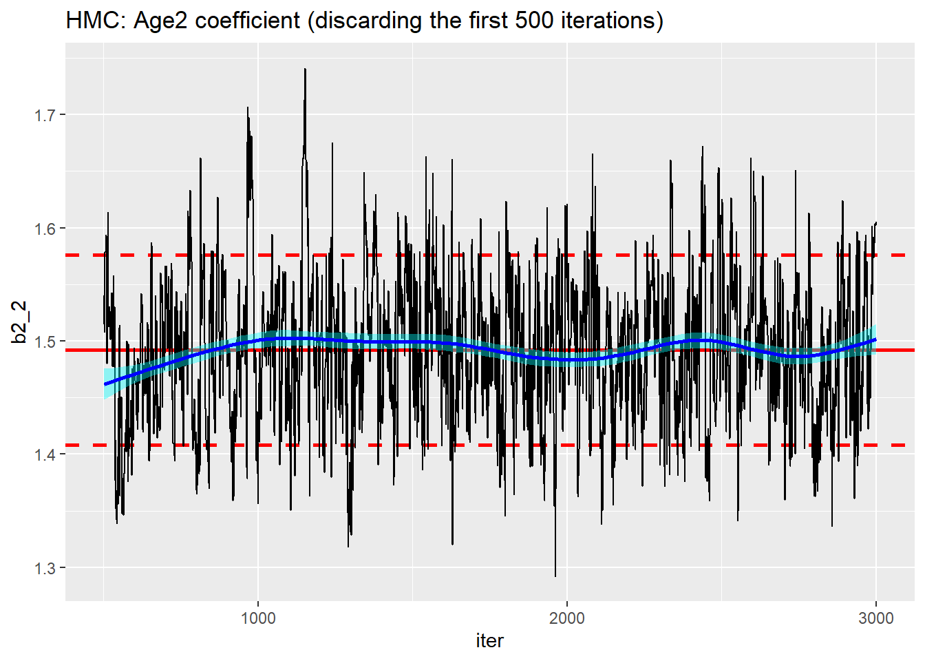
There is a good algorithm in there somewhere, but it is not automatic.
A spanner in the works
My first time run of length 3000 ran in 20 seconds!!
Remember, it took 75 seconds to run 1000 iterations and I put this down to initialising the AD. Perhaps that was not correct. Could it be that the slow time for the shorter run was due to poor tuning of the algorithm in the correspondingly shorter warm-up.
I tried setting the nburnin parameter of runMCMC() to 500. This had the effect to discarding the first 500 iterations, but the warm-up was still of length 1000.
# --- read the result -----------------------------------------
readRDS(file.path( home, "data/dataStore/testHMC07.rds")) %>%
  nimble_to_df() -> simDF

trace_plot(simDF, b2_2, iter) +
  labs(title="HMC: Age2 coefficient (with a burn-in of 500)")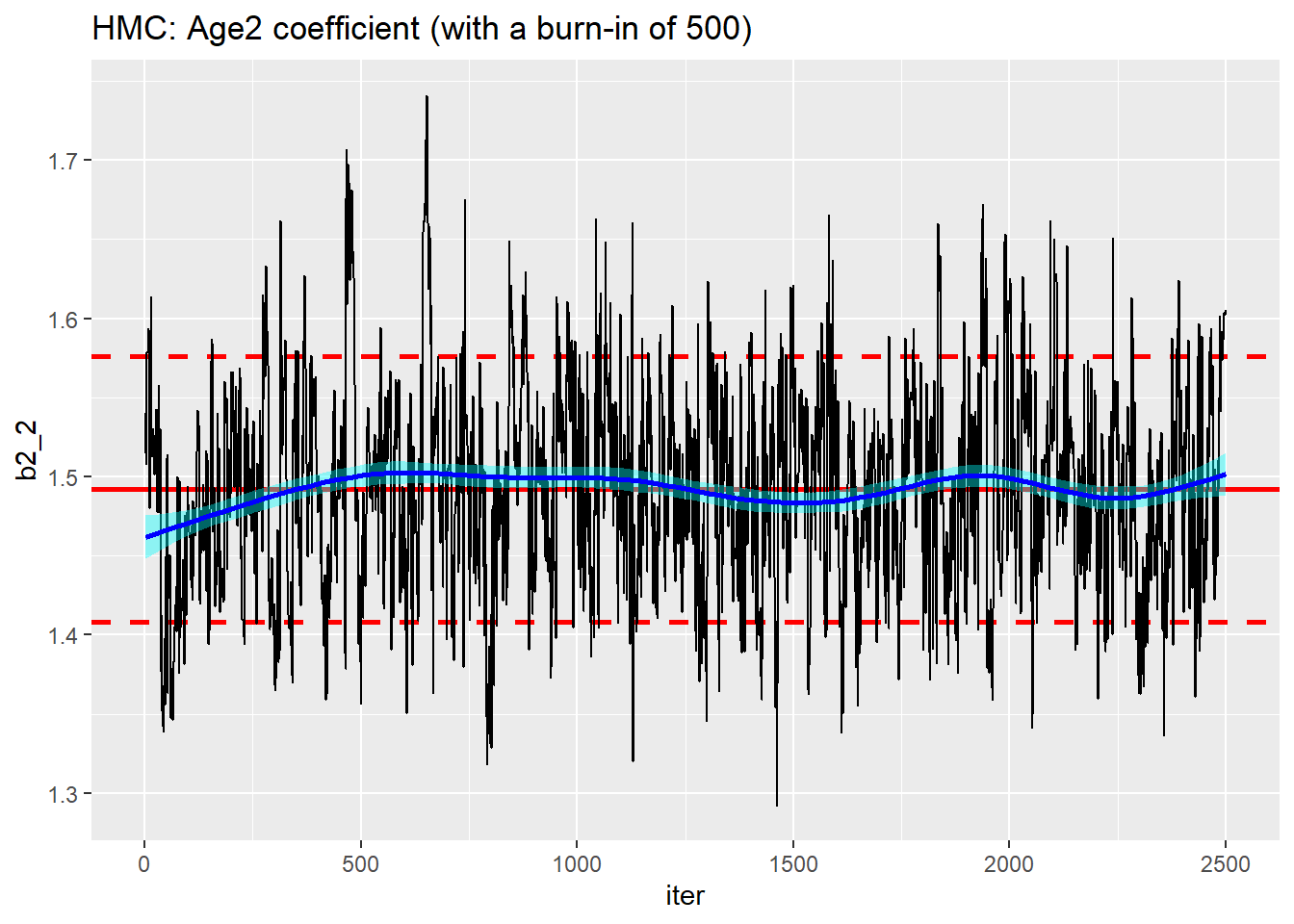
As far as I can tell, there is no way of requesting a longer warm-up. The length seems to be set automatically.
How about MCMC
One final comparison, I ran the default MCMC with random walk samplers for all of the parameters. I decided on a run of 10,000 with the first 5,000 discarded.
Mixing is still quite poor although the algorithm has found the right region.
# --- read the result -----------------------------------------
readRDS(file.path( home, "data/dataStore/testMCMC08.rds")) %>%
  nimble_to_df() -> simDF

trace_plot(simDF, b2_2, iter) +
  labs(title="MCMC: Age2 coefficient (median and 80% interval)")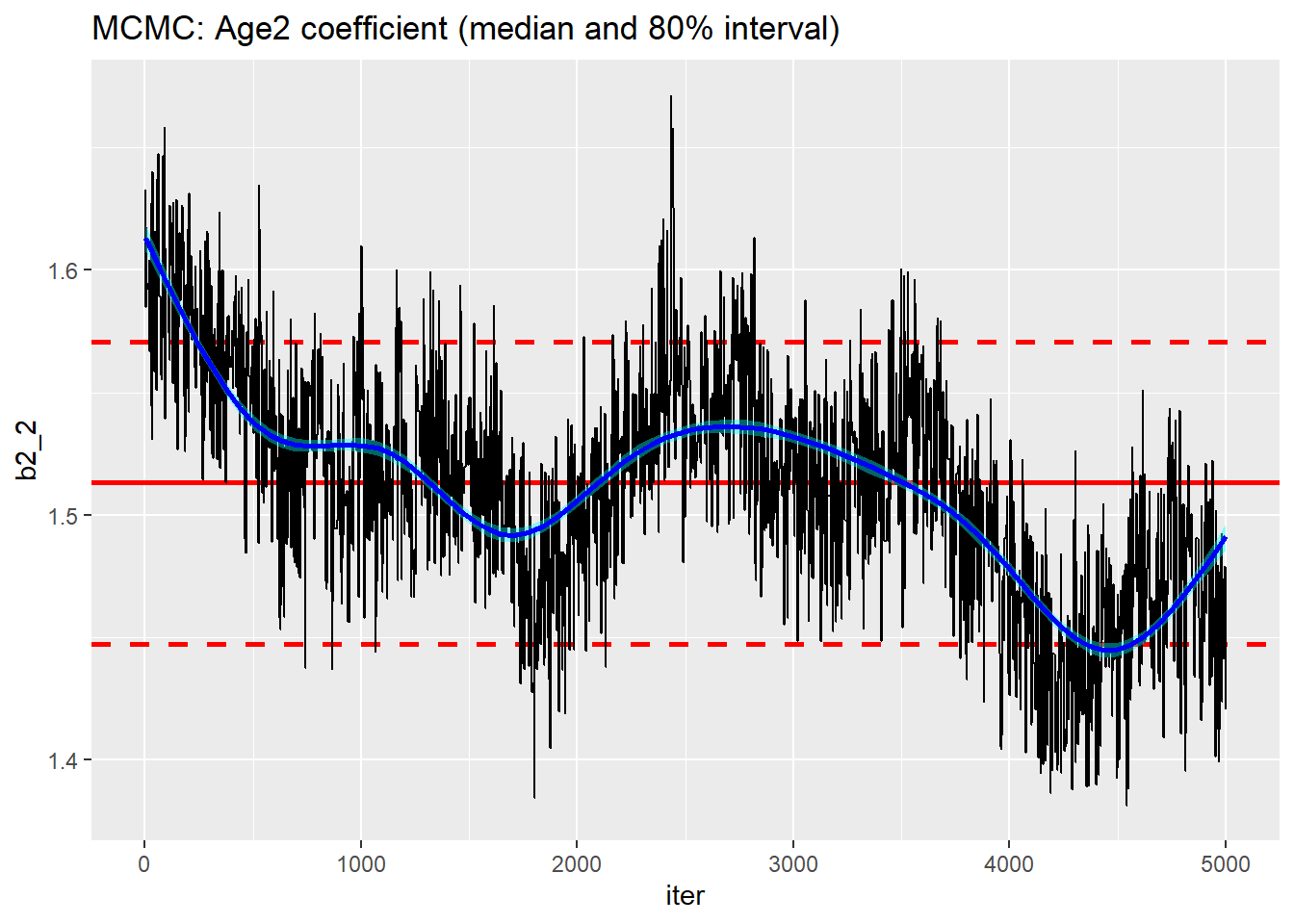
On the plus side, this run took under 4 seconds. This means that in the 20 seconds that HMC took to give me 2500 usable simulations, I could have run an MCMC chain of length 50,000 and discarded the first 5,000 and thinned by 18 to leave me with 2,500 usable simulations. I tried it and it did take about 20 seconds.
# --- read the result -----------------------------------------
readRDS(file.path( home, "data/dataStore/testMCMC09.rds")) %>%
  nimble_to_df() -> simDF

trace_plot(simDF, b2_2, iter) +
  labs(title="MCMC: Age2 coefficient (50,000 thinned by 18)")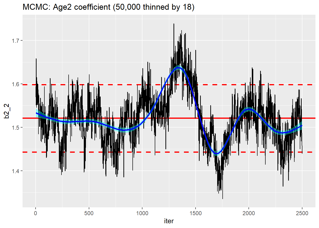
Nice idea but the mixing is still terrible, far worse than the corresponding HMC run.
I know that I could centre the x’s, use a block sampler for the correlated parameters and tune the standard deviation of the random walk, but the fundamental problem remains; RW Metropolis-Hastings is not a great algorithm.
Conclusions
So back to where I started with my conclusions
- I remain optimistic that HMC will make nimble a more competitive option for Bayesian model fitting
- nimble’s default random walk MCMC is not a great algorithm
- No Monte Carlo algorithm is ever fully automatic
- Entering the explanatory variables as constants rather than data overcomes the dynamic indexing problem.
- The dynamic indexing and the dummy variables parameterisations gave similar results in similar run-times.
- Playing with a beta version of a package is a process of trial and error
- You need to be very careful with Object Orientated Programming (OOP) software, because it is in the nature of OOP that objects can change internally without you realising, which means that a second run of apparently identical code will not necessarily give the same results as a first run. Be careful.
- The long run times that I experienced with some analyses seem to have been due to too short a warm-up leading to a poorly tuned algorithm. It was not a problem of setting up the automatic differentiation (A)D as I initially suspected.
- Given the importance of tuning an algorithm to each specific problem,
nimbleneeds to make it easy for the user to control the algorithm.