Methods: Nimble HMC
Introduction
In my methods post entitled “R Software for Bayesian Analysis”, I discussed the problem of fitting Bayesian models using various R packages including, R2OpenBUGS, nimble, rstan and greta. nimble is particularly interesting because it is specifically written for use in R. It is very fast, but its default algorithm is based on Gibbs sampling with a series random walk Metropolis-Hastings samplers and this algorithm can mix poorly, leading to very long run times.
Earlier this summer, nimble released a beta version that includes the same Hamiltonian Markov Chain (HMC) sampler that has made stan so popular. In this post, I will try HMC in nimble.
Reading the data
In my previous post, I modelled ONS (Office of National Statistics) data on deaths due to alcohol in the UK. The data can be downloaded as an Excel workbook from https://www.ons.gov.uk/peoplepopulationandcommunity/healthandsocialcare/causesofdeath/datasets/alcoholspecificdeathsintheukmaindataset.
I used a version of the data that covered the period 2001 to 2020. These data are updated annually, so beware if you download the latest dataset, it might have changed.
Previously, I cleaned the downloaded Excel file and saved the data in rds format. My cleaning script is included in the earlier post.
library(tidyverse)

# --- paths on my desktop --------------------------------------
home     <- "C:/Projects/sliced/methods/methods_bayes_software"
filename <- "data/rData/alc.rds"

# --- read the clean data --------------------------------------
alcDF <- readRDS( file.path(home, filename))
Let’s try nimble HMC
What follows uses the beta version of nimble downloaded from github on 26 September 2022.
# install from github
remotes::install_github("nimble-dev/nimble",
                        ref="AD-rc0",
                        subdir="packages/nimble",
                        quiet=TRUE)
# install the HMC package
remotes::install_github("nimble-dev/nimbleHMC", subdir = "nimbleHMC")
For more details of HMC in nimble, there is a draft manual that can be found at https://r-nimble.org/ADuserManual_draft/chapter_AD.html.
I discovered that I needed to update all of the other packages in my library before I could install the beta version of nimble.
Preparing the model code
nimble uses the BUGS language with a few tweaks and additions. For my first attempt, I use the same model as I had previously.
library(nimble)

# --- Model code as used previously ------------------------------
nimbleCode( {
  for( i in 1:560 ) {
    log(mu[i]) <- b0 + b1*year[i] + b2[age[i]] + b3*gender[i] + offset[i]
    deaths[i] ~ dpois(mu[i])
  }
  b0 ~ dnorm(0, 0.0001)
  b1 ~ dnorm(0, 0.0001)
  b2[1] <- 0.0
  for(j in 2:14) {
    b2[j] ~ dnorm(0, 0.0001)
  }
  b3 ~ dnorm(0, 0.0001)
} )                       -> modelCode
This code worked fine for MCMC with Gibbs sampling, but unfortunately there is a problem with HMC. In its current form, nimble cannot calculate derivatives for terms that include dynamic indexing, i.e. b2[age[i]].
There are two alternatives, use MCMC for b2 and HMC for the other parameters, or expand the age term as a set of dummy variables. I’ll try the later approach first.
# --- create dummy variables for age -----------------------------
alcDF %>%
  mutate(dummy = paste0("age", as.numeric(age)),
         value = 1) %>%
  pivot_wider(names_from  = dummy,
              values_from = value,
              values_fill = 0) %>%
  ungroup() %>%
  select(-age, -age1) %>%
  print() -> dummyAgeDF
## # A tibble: 560 × 17
## year gender deaths pop age2 age3 age4 age5 age6 age7 age8 age9
## <dbl> <chr> <dbl> <dbl> <dbl> <dbl> <dbl> <dbl> <dbl> <dbl> <dbl> <dbl>
## 1 2020 male 4 20.8 0 0 0 0 0 0 0 0
## 2 2020 female 5 23.5 0 0 0 0 0 0 0 0
## 3 2020 male 23 21.1 1 0 0 0 0 0 0 0
## 4 2020 female 23 21.3 1 0 0 0 0 0 0 0
## 5 2020 male 115 21.3 0 1 0 0 0 0 0 0
## 6 2020 female 71 21.5 0 1 0 0 0 0 0 0
## 7 2020 male 272 21.7 0 0 1 0 0 0 0 0
## 8 2020 female 159 22.1 0 0 1 0 0 0 0 0
## 9 2020 male 457 21.8 0 0 0 1 0 0 0 0
## 10 2020 female 232 22.2 0 0 0 1 0 0 0 0
## # … with 550 more rows, and 5 more variables: age10 <dbl>, age11 <dbl>,
## # age12 <dbl>, age13 <dbl>, age14 <dbl>Here is the model code rewritten in terms of the dummy variables.
# --- Model code with dummy variables ---------------------------
nimbleCode( {
  for( i in 1:560 ) {
    log(mu[i]) <- b0 + b1*year[i] +
      b2[ 2]*age2[i]  + b2[ 3]*age3[i]  + b2[ 4]*age4[i] +
      b2[ 5]*age5[i]  + b2[ 6]*age6[i]  + b2[ 7]*age7[i] +
      b2[ 8]*age8[i]  + b2[ 9]*age9[i]  + b2[10]*age10[i] +
      b2[11]*age11[i] + b2[12]*age12[i] + b2[13]*age13[i] +
      b2[14]*age14[i] + b3*gender[i] + offset[i]
    deaths[i] ~ dpois(mu[i])
  }
  b0 ~ dnorm(0, 0.0001)
  b1 ~ dnorm(0, 0.0001)
  b2[1] <- 0.0
  for(j in 2:14) {
    b2[j] ~ dnorm(0, 0.0001)
  }
  b3 ~ dnorm(0, 0.0001)
} )                       -> modelCode
Creating a Model Object
In nimble a model object is a combination of the model code, the data and the initial values. The data and initial values are placed in a list.
The HMC algorithm in stan does not require initial values, stan finds an approximate solution during its warm-up. The manual is not clear, but it suggests that nimble does need initial values, so I use the same crude initial values that I had previously.
# --- list containing the data -------------------------
nimbleData <- list( deaths = dummyAgeDF$deaths,
                    offset = log(dummyAgeDF$pop),
                    year   = dummyAgeDF$year - 2001,
                    gender = as.numeric( dummyAgeDF$gender == "male"),
                    age2     = dummyAgeDF$age2,
                    age3     = dummyAgeDF$age3,
                    age4     = dummyAgeDF$age4,
                    age5     = dummyAgeDF$age5,
                    age6     = dummyAgeDF$age6,
                    age7     = dummyAgeDF$age7,
                    age8     = dummyAgeDF$age8,
                    age9     = dummyAgeDF$age9,
                    age10    = dummyAgeDF$age10,
                    age11    = dummyAgeDF$age11,
                    age12    = dummyAgeDF$age12,
                    age13    = dummyAgeDF$age13,
                    age14    = dummyAgeDF$age14 )

# --- initial values -----------------------------------
nimbleInits <-
  list( b1=0, b2=c( NA, rep(0,13)), b3=0)
Notice that I have not centred the covariates. Mean centring usually improves mixing for Gibbs samplers, but should not matter as much for HMC.
Next, I combine the components and add a new argument that tells nimble to build the derivatives. nimble uses an automatic differentiation (AD) package that has been around for a while. The package is called CppAD and as the name suggests is written in C++.
Once defined, I compile the model to produce the necessary C code.
# --- create the model ---------------------------------
nimbleModel(
  code  = modelCode,
  data  = nimbleData,
  inits = nimbleInits,
  # --- ADDITION: add derivatives
  buildDerivs = TRUE ) -> model

# --- Compile the model ---------------------------------
modelCompiled <- compileNimble(model)
Building the HMC sampler
Next the samplers are allocated in a build phase. Where before I used buildMCMC(), the new builder is buildHMC() which is found in the nimbleHMC package.
# --- select the samplers ---------------------------------
library(nimbleHMC)

modelHMC <- buildHMC(model)
Once samplers have been chosen, the algorithm needs to be compiled and linked to the previously compiled model code.
# --- compile the sampling algorithm ----------------------
hmcCompiled <- compileNimble(modelHMC, project=model)
hmcCompiled points to the full C code needed needed for the analysis.
Run
When the compiled C program is run, the number of iterations and chains must be specified. As this is a demonstration, I will only run one chain. My earlier post describes how multiple chains can be run in parallel. A seed is set for reproducibility.
I have not specified the burn-in although the manual implies that you should. HMC has a warm-up period during which the algorithm is tuned, but no burn-in in the sense of MCMC. As an experiment, I tried without a specified burn-in and it worked fine.
# --- run the compiled nimble code ----------------------
runMCMC(
  mcmc    = hmcCompiled,
  niter   = 1000,
  setSeed = 1832
  )  %>%
  saveRDS( file.path( home, "data/dataStore/alcNimbleHMC01.rds")) %>%
  system.time()
The sampling took 11.25 seconds. This compares with about 3.5 seconds needed by nimble’s MCMC algorithm to run 1500 simulations and discard the first 500. HMC is always slower because it needs to calculate the exact derivatives of the log posterior, the hope is that this will be balanced by better mixing and much faster convergence.
Extract the results
The structure returned by runMCMC() is just a matrix, but a little wrangling is needed to get it into a more usable format. My function nimble_to_df() does the job. The code for this function is in the previous post.
library(MyPackage)

# --- read the result -----------------------------------------
results <- readRDS(file.path( home, "data/dataStore/alcNimbleHMC01.rds"))

# --- read the results for the example ------------------------
simDF <- nimble_to_df(results)

# --- show the results ----------------------------------------
print(simDF)
## # A tibble: 1,000 × 19
## chain iter b0 b1 b2_1 b2_2 b2_3 b2_4 b2_5 b2_6 b2_7 b2_8
## <fct> <int> <dbl> <dbl> <dbl> <dbl> <dbl> <dbl> <dbl> <dbl> <dbl> <dbl>
## 1 1 1 -1.57 0.0147 0 1.37 2.39 3.14 3.70 4.06 4.24 4.33
## 2 1 2 -1.57 0.0147 0 1.37 2.39 3.14 3.70 4.06 4.24 4.33
## 3 1 3 -1.57 0.0141 0 1.37 2.39 3.15 3.69 4.06 4.25 4.30
## 4 1 4 -1.57 0.0143 0 1.36 2.41 3.12 3.69 4.06 4.26 4.32
## 5 1 5 -1.57 0.0143 0 1.36 2.41 3.12 3.69 4.06 4.26 4.32
## 6 1 6 -1.57 0.0148 0 1.37 2.41 3.12 3.69 4.05 4.25 4.33
## 7 1 7 -1.66 0.0137 0 1.46 2.52 3.22 3.78 4.17 4.35 4.42
## 8 1 8 -1.66 0.0142 0 1.48 2.52 3.22 3.78 4.14 4.34 4.42
## 9 1 9 -1.66 0.0142 0 1.48 2.52 3.22 3.78 4.14 4.34 4.42
## 10 1 10 -1.68 0.0144 0 1.46 2.52 3.26 3.82 4.19 4.37 4.44
## # … with 990 more rows, and 7 more variables: b2_9 <dbl>, b2_10 <dbl>,
## # b2_11 <dbl>, b2_12 <dbl>, b2_13 <dbl>, b2_14 <dbl>, b3 <dbl>Visualise the results
Now that the samples are in a tibble, the chain can be inspected. By way of illustration, I show a trace plot of the year coefficient, b1. The code for the trace_plot() function is also available in the earlier post.
# --- trace plot of b1 -------------------------------
trace_plot(simDF, b1, iter) +
  labs(title="HMC: Year coefficient (median and 80% interval)")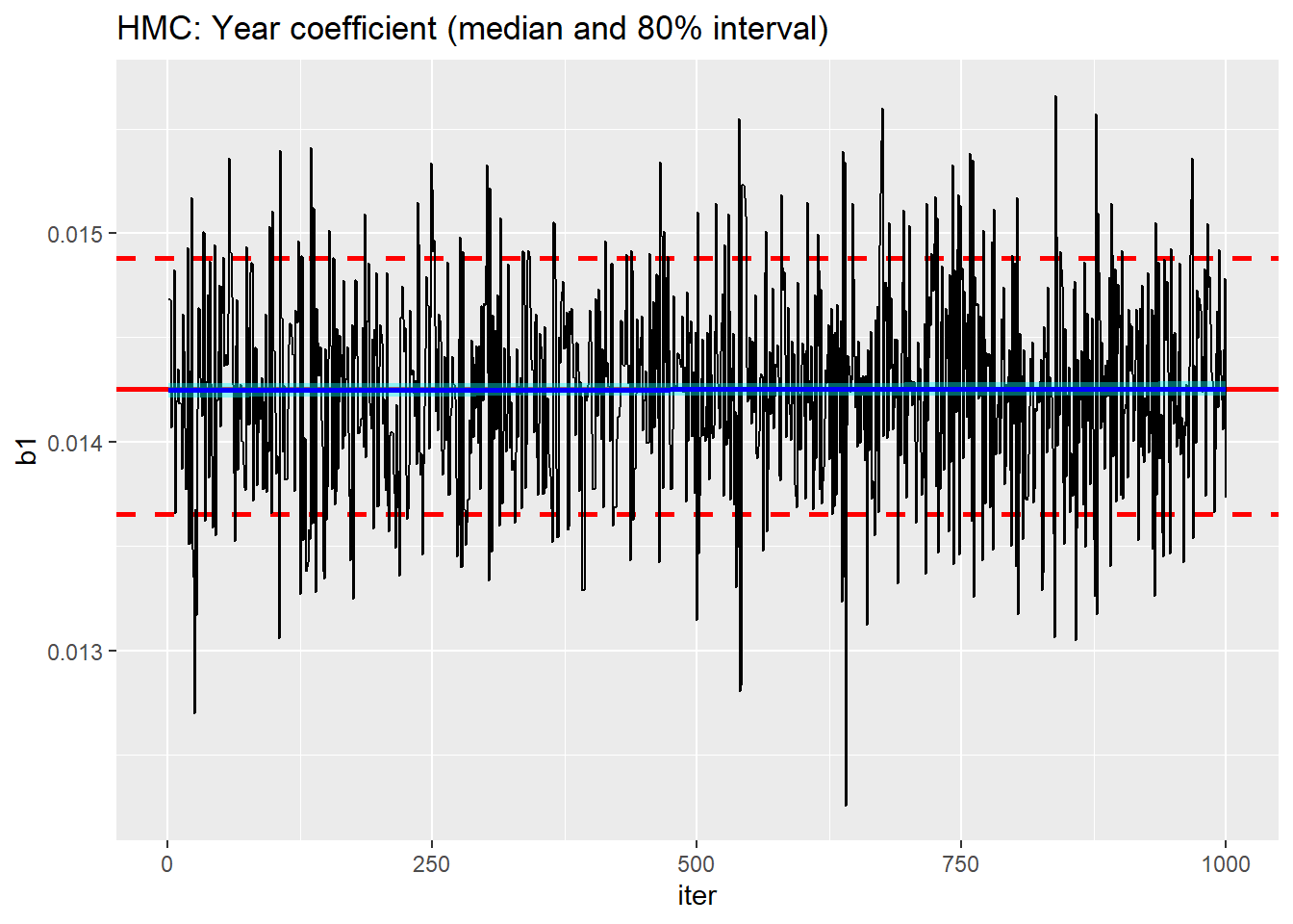
For comparison, I went to my archive and extracted the chain that I created for my previous post using nimble’s default MCMC sampler.
readRDS(file.path( home, "data/dataStore/alcNimble01.rds")) %>%
  nimble_to_df() %>%
  trace_plot(b1, iter) +
  labs(title="MCMC: Year coefficient (median and 80% interval)")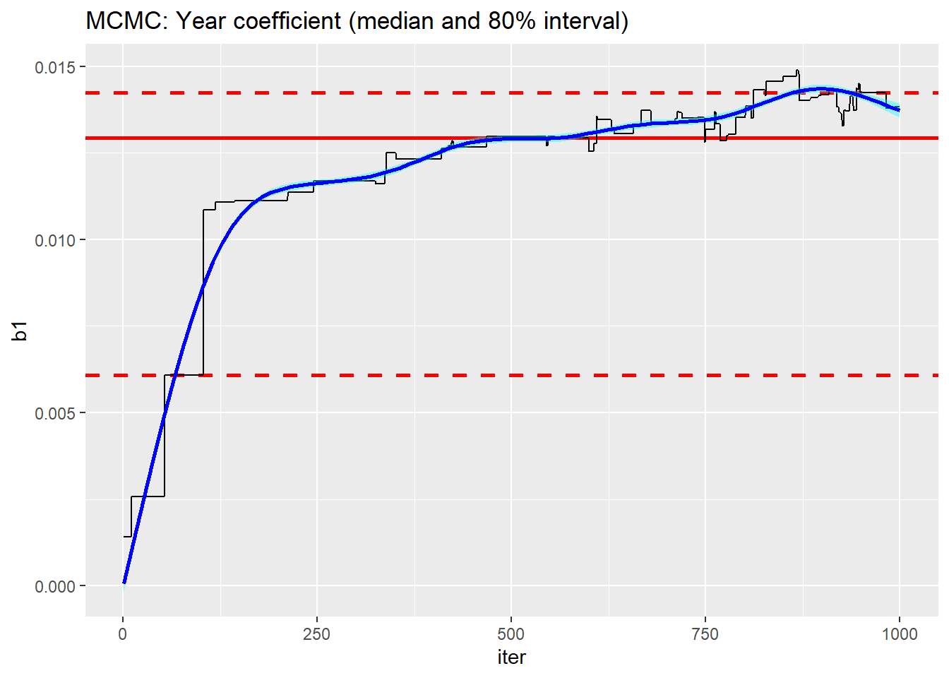
No competition, HMC converges much quicker.
Half and Half
I wanted to try HMC for b0, b1 and b3 together with a random walk block sampler for b2. In theory this should overcome the problem of the dynamic indexing of b2. However, I could not get this to work and there is not enough information in the draft manual to make it clear how it should be done.
In truth, I am not convinced that this is a good idea anyway. HMC is slow but only requires a short run, while MCMC is fast but needs a long run. Will the mixture be a medium length run of a medium speed algorithm, or will we now need a long, slow run? It is unclear to me whether combining MCMC and HMC is a good option.
Conclusions
It is early days and nimbleHMC still needs work, but it looks very promising. The developers have addressed a major weakness in nimble and turned it into a serious option for Bayesian model fitting. The test will be how well it scales to larger problems and whether nimble can compete with stan in terms of speed.
The remaining issue, as I see it, is that nimble is so versatile that the range of its options will prove off-putting to users who are not relatively expert in R. There is a parallel here with mlr3 a competitor of tidymodels that I have used in other of my posts. In my opinion, mlr3 is the better option for building machine learning pipelines, but like nimble it relies on OOP with R6 and this fact is not completely hidden from the user. Somehow, both packages need to simplify their interfaces, while maintaining their amazing flexibility and that will not be easy.