Methods: MCMC Algorithms
Introduction
Markov Chain Monte Carlo (MCMC) Samplers are ways of drawing representative values from a target distribution. In this post I will develop MCMC sampling from scratch and illustrate some of the most popular algorithms with simple R code. The key to understanding the approach lies in the name; Monte Carlo says that the values will be drawn by a random process and Markov Chain says that each sampled value will be dependent on the previous value.
The algorithms are usually applied to Bayesian problems in which the target is the posterior distribution of a model parameter.
MCMC is quite general; the target distribution can be continuous or discrete, one-dimensional or multi-dimensional. To simplify the explanation, I start with a one-dimensional, discrete target distribution of a parameter that I call \(\theta\).
Recognised Distributions
On rare occasions the pattern of the probabilities of different values of \(\theta\) will be recognised as following a standard distribution. For example, suppose that the target distribution is defined over the integer values 0 to 4 with probabilities,
(0) 0.4096, (1) 0.4096, (2) 0.1536, (3) 0.0256, (4) 0.0016
You might recognise this pattern as a binomial distribution with n=4 and p=0.2, in which case there is no need for MCMC because the R function rbinom() does the job.
# --- seed for reproducibility -----------
set.seed(3491)
# --- 5000 random values -----------------
theta <- rbinom(5000, size=4, prob=0.2)
# --- table of sample proportions --------
table(theta)/5000
## theta
## 0 1 2 3 4
## 0.4138 0.4056 0.1478 0.0314 0.0014The proportions vary from the target, but only by chance and the more samples that are taken, the closer will be the approximation.
Metropolis-Hastings
Assuming that the target distribution is not recognised, the best option is an MCMC algorithm.
The MCMC algorithm must create an ordered sequence of values (a chain) and the way to ensure that the chain represents the target distribution is to use the correct transition probabilities for generating one value from its predecessor. We need to pick appropriate values for quantities such as, \(T(3 | 2) = P(\theta_i=3 | \theta_{i-1}=2)\), which is the probability of sampling the value 3 when the previous value was 2.
Take an arbitrary pair of consecutive values, say they are 3 and 1. If the entire chain were written in reverse order, it would still represent the same target distribution, so (3 followed by 1) and (1 followed by 3) should be equally common in the chain, i.e. P(3,1)=P(1,3). It follows that \[ P(3,1) = P(3).T(1 | 3) = P(1,3) = P(1). T(3|1) \] In words, the probability of being at 3 and transitioning to 1 equals the probability of being at 1 and transitioning to 3.
This is the fundamental relationship of MCMC that links the transition probabilities, T, to the target distribution, P. Generally,
\[
P(a) T(b | a) = P(b) T(a | b)
\]
This relationship holds for any consecutive pair of values (a,b) and is sometimes called detailed balance. The MCMC algorithm must obey this rule.
Suppose that the target distribution is (0) 0.2, (1) 0.3, (2) 0.1, (3) 0.3, (4) 0.1
library(tidyverse)
theme_set(theme_light())

# --- histogram of the taregt distribution -----------------------
tibble( x = 0:4,
        P = c(0.2, 0.3, 0.1, 0.3, 0.1)) %>%
  ggplot( aes(x=x, y=P)) +
  geom_bar( stat="identity", fill="steelblue") +
  labs(title="Target distribution for the example")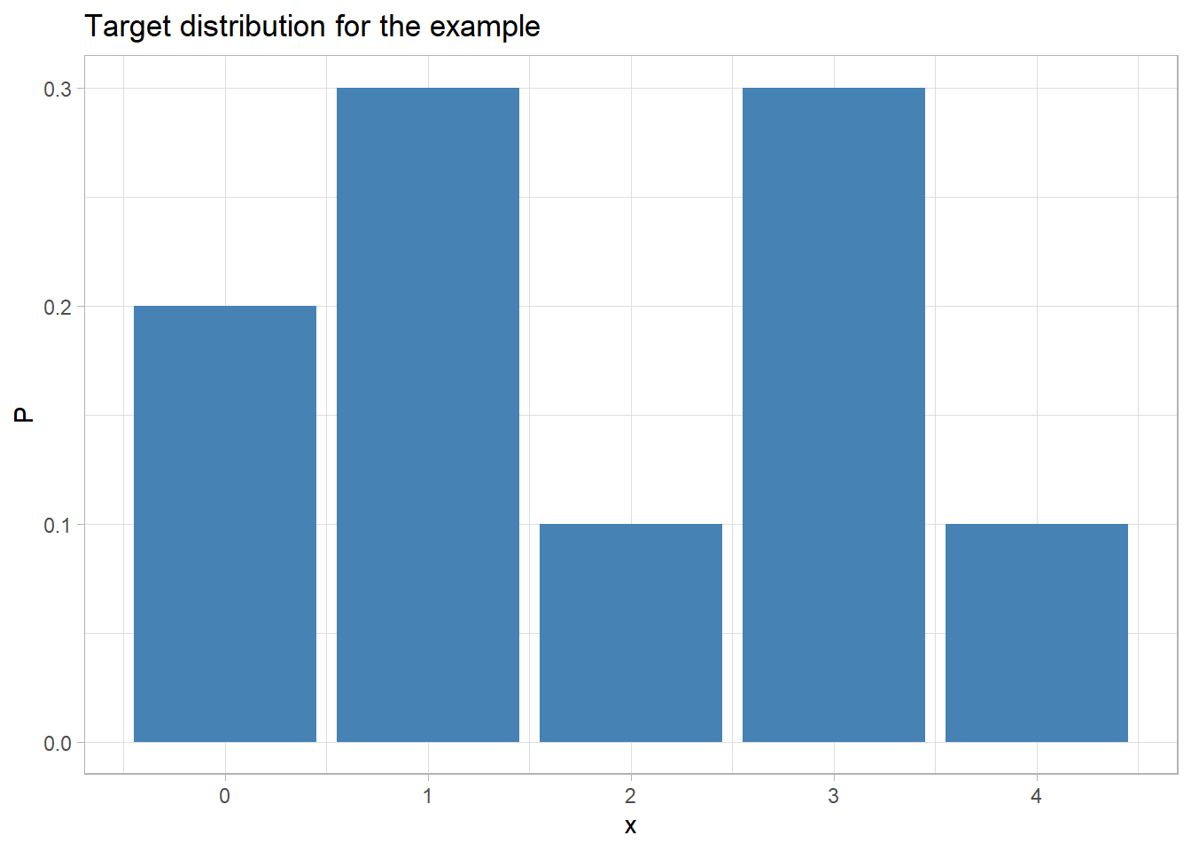
Imagine that the chain is currently at 1, with equal probability, a potential next value is chosen; it could be 0, 2, 3 or 4. This proposal will either be accepted or rejected, and if it is rejected the chain will have to stay at 1. So the consecutive pair could be any of (1,0), (1,1), (1,2), (1,3), (1,4).
Suppose that starting from 1, we randomly select 0 as the potential move. We know that for our target distribution, P(0)=0.2 and P(1)=0.3, so detailed balance tells us that \[ 0.3 T(0 | 1) = 0.2 T(1 | 0) \] This relationship simultaneously constrains the transition probabilities for T(0|1) and the reverse T(1|0). All we need to do, is to choose any pair of transition probabilities T(0|1) and T(1|0) that satisfy this relationship. For example, T(0|1)=0.2 and T(1|0)=0.3 or T(0|1)=0.4 and T(1|0)=0.6, etc.
The larger the pair of probabilities, the more likely the chain is to move and we want to move in order to cover the distribution as quickly as possible, so the optimum choice is T(1|0)=1 and T(0|1)=2/3.
We can repeat this argument for any pair of values. Detailed balance tells us that \[ \frac{P(a)}{P(b)} = \frac{T(a | b)}{T(b | a)} \] and the optimum choice will be \[ T(a|b) = min\left\{ 1, \frac{P(a)}{P(b)}\right\} \ \ \text{and} \ \ T(b|a) = min\left\{ 1, \frac{P(b)}{P(a)}\right\} \]
Let’s code this algorithm
# --- Possible values
domain <- c(0, 1, 2, 3, 4)
# --- target distribution = probabilities of each value
prb <- c( 0.2, 0.3, 0.1, 0.3, 0.1)

# --- seed for reproducibility
set.seed(8407)
# --- space for 5000 simulations
theta <- rep(0, 5000)
# --- start with a random value
theta[1] = sample(domain, size=1)
# --- loop to complete the chain
for( i in 2:5000) {
  # --- Identify all possible moves i.e. not theta[i-1]
  possibleMoves <- domain[ !(domain %in% theta[i-1]) ]
  # --- select one move at random
  move <- sample(possibleMoves, size=1)
  # --- Calculate the acceptance probability,
  #     n.b. because 0 is a possibility, P(theta=1) = prb[2]
  acceptProb <- min( 1, prb[move+1]/prb[theta[i-1]+1])
  # --- Randomly Move or Stay with acceptProb
  theta[i] <- ifelse(runif(1) < acceptProb, move, theta[i-1])
}
# --- Inspect the first 20 values
print(theta[1:20])
## [1] 0 4 0 1 3 1 2 1 1 3 3 1 3 1 3 1 0 3 3 3# --- frequencies of each value in the chain
table(theta)/5000## theta
## 0 1 2 3 4
## 0.2006 0.2922 0.0966 0.3116 0.0990The algorithm reproduces the target distribution quite well. The longer the chain the closer the proportions will be to the target.
There is one final refinement to the algorithm. I started by choosing the potential move from all possible moves with equal probability. This works fine for a distribution with a small number of possible moves, but for distributions defined over a large domain, it can be easier to restrict the set of possible moves, for example, to favour local proposed moves over longer steps.
We can adapt the algorithm by writing, \[ T(b|a) = G(b|a) A(b|a) \] where G(b|a) is the proposal probability that we control, i.e. the probability that we propose a move from a to b, and A(b|a) is the probability that we accept that move.
In this more general case, detailed balance becomes \[ P(a) G(b|a) A(b|a) = P(b) G(a | b) A(a | b) \] and the acceptance probability A is obtained from \[ A(b|a) = min\left\{ 1, \frac{P(b) G(a|b)}{P(a) G(b|a)}\right\} \] This is the full Metropolis-Hastings Algorithm, which is illustrated below for the case where I choose a proposal that is either 1 higher or 1 lower than the current value.
# My Proposal Rule: Move up or down 1 provided stay within the domain
# i.e. from 2 propose move to 1 or 3 with equal probability
# but from 4 may only propose a move to 3
#
# --- proposal probabilities G ..
G <- matrix( c(0, 0.5, 0, 0, 0,
               1, 0, 0.5, 0, 0,
               0, 0.5, 0, 0.5, 0,
               0, 0, 0.5, 0, 1,
               0, 0, 0, 0.5, 0), nrow=5)

# --- Possible values
domain <- c(0, 1, 2, 3, 4)
# --- target distribution = probabilities of each value
prb <- c( 0.2, 0.3, 0.1, 0.3, 0.1)

# --- seed for reproducibility
set.seed(3407)
# --- space for 5000 simulations
theta <- rep(0,5000)
# --- start with a random value
theta[1] = sample(domain, size=1)
# --- loop to complete the chain
for( i in 2:5000) {
  # --- Identify all possible moves .. +1 or -1
  possibleMoves <- c( theta[i-1]-1, theta[i-1]+1)
  possibleMoves <- possibleMoves[ possibleMoves >= 0 & possibleMoves <= 4]
  # --- select one potential move at random
  # note oddity in R's sample() function means it cannot be used
  # see help(sample) for details ... use sample.int() instead
  move <- possibleMoves[sample.int(length(possibleMoves), size=1)]
  # --- domain starts at 0 while subscripts start at 1
  from <- theta[i-1] + 1
  to   <- move + 1
  # --- Calculate the acceptance probability
  acceptProb <- min( 1, prb[to]*G[to, from]/(prb[from]*(G[from, to])))
  # --- Randomly Move or Stay with probability=acceptProb
  theta[i] <- ifelse(runif(1) < acceptProb, move, theta[i-1])
}
# --- Inspect the first 20 values
print(theta[1:20])
## [1] 0 1 1 1 2 3 3 3 2 1 0 1 0 0 0 1 1 1 0 1# --- frequencies of each value in the chain
table(theta)/5000## theta
## 0 1 2 3 4
## 0.2106 0.3072 0.0952 0.2852 0.1018Perhaps not quite as good an algorithm, but the target distribution is still being reproduced. The poorer performance is due to taking longer to move from one end of the distribution to the other, when only single steps are allowed.
Slice Sampling
Metropolis-Hastings is a flexible algorithm that can usually be tuned by the choice of the proposal distribution, G, to sample parameter values in an efficient way, but it is not the only option. A powerful alternative is an algorithm known as Slice Sampling.
Given the current sample value \(\theta\), choose a random value, u, in the range from 0 to P(\(\theta\)). Next, identify all values in the domain that have a probability of at least u and choose one at random. The chosen value is taken as the next value in the chain.
Here is a sample from our target distribution drawn by Slice sampling.
# --- SLICE sampling -------------------------------------
#
# target distribution
prb <- c( 0.2, 0.3, 0.1, 0.3, 0.1)
domain <- c(0, 1, 2, 3, 4)
set.seed(3929)

# --- space to save 5000 samples
theta <- rep(0,5000)
# --- arbitrary initial value
theta[1] = sample(domain, size=1)
# --- loop to generate the sample
for( i in 2:5000 ) {
  # --- random value in range (0, P(x[i-1]))
  u <- runif(1, 0, prb[theta[i-1]+1])
  # --- all potential values that have prob >= u
  set <- which( prb >= u )
  # --- choose a value at random from those with prob > u
  theta[i] <- set[sample.int(length(set), size=1)] - 1
}
# --- inspect the results
table(theta)/5000
## theta
## 0 1 2 3 4
## 0.1954 0.2940 0.0992 0.3056 0.1058Slice sampling works well for this example.
Generalising to Continuous Distributions
When the target distribution is continuous, the algorithms take the same form but with probability densities (the heights of the density curves) replacing the discrete probabilities.
For Slice sampling with continuous distributions, careful programming is needed to identify the set of values with probability greater or equal to u in an efficient way.
Gibbs sampling
The Metropolis-Hastings and Slice sampling algorithms work in any number of dimensions, but in high dimensions, they becomes very inefficient. It is increasingly difficult to propose moves for the Metropolis-Hastings algorithm that will not be rejected and it is increasingly difficult to identify the set of potential values (the slice) for Slice sampling.
Gibbs sampling offers a way around this problem by updating each parameter (dimension) in turn, with the remaining parameters held fixed. It is generally the case that Gibbs sampling takes longer to cover a multi-dimensional posterior, but it only ever requires one dimensional updates, which are usually easier to create.
Gibbs sampling works well when there is low correlation between parameters but can become very slow to converge to the target when pairs of parameters are highly correlated. In such situations, it may be necessary to re-parameterise the problem, or to update the correlated parameters as a block.
Hamiltonian Markov Chain (HMC)
As already noted, Gibbs Sampling performs well provided the parameters of a model are not highly correlated. When they are, Gibbs samplers tends to get struck in one part of the posterior. It is not uncommon to hear stories of models fitted by Gibbs Sampling, where the software converges to the correct multi-dimensional target but only after hundreds of thousands of iterations taking days of computation.
HMC is a form of MCMC that is capable of updating all parameters at the same time, so it is much less affected by the correlation between parameters. The computation for each iteration takes longer, but far fewer iterations are needed. The secret of HMC is that it uses both the probability density of the target distribution and the derivative of that probability density. Rather like gradient descent in optimisation problems, the derivative tells HMC how to change the parameters in order to cover the target distribution more efficiently.
HMC can only be used when the parameters have a continuous distribution with smooth derivatives and it is only accurate, when those derivatives are precise; numerical differentiation is not good enough.
There are two ways of motivating the HMC algorithm, by analogy with the path of a particle moving over a multi-dimensional surface, or as an auxiliary variable method in which extra parameters are added to the model to make it easier to simulate. In the physical analogy, the auxiliary variables represent the velocity of the particle.
Let’s suppose that \(\theta\) is a multi-dimensional parameter; in the physical analogy, the values of \(\theta\) correspond to the co-ordinates of the particle. \(\phi\) is the auxiliary variable, it has the same dimension as \(\theta\) and represents the components of the velocity of the particle.
The joint distribution of \(\phi\) and \(\theta\) is \[ p(\phi, \theta) = p(\phi | \theta) p(\theta) \] Since \(\phi\) is not inherent in the original problem, \(p(\phi | \theta)\) can be chosen in any way that simplifies the joint sampling and once \(\phi\) and \(\theta\) have been simulated, the values of \(\phi\) can be discarded to leave a value \(\theta\) drawn from the target distribution \(p(\theta)\).
If we take minus the log of this expression, we get something that is usually called H (H is analogous to the Hamiltonian of classical dynamics and can be used to calculate the path of a particle given its position and velocity) \[ H(\phi, \theta) = -log\left[p(\phi, \theta)\right] = -log\left[p(\phi | \theta)\right] - log\left[p(\theta)\right] \] Hamilton’s equations of motion update the values of \(\phi\) and \(\theta\) in time, t, according to the following rule. \[ \frac{\partial \phi}{\partial t} = \frac{\partial H}{\partial \theta} \frac{\partial \theta}{\partial t} = -\frac{\partial H}{\partial \phi} \]
So the path of \(\theta\) and \(\phi\) can be traced for a fixed time t, before \(\phi\) is discarded. In the physical analogy, what happens is that the particle moves over the surface defined by minus the log of the target density, gaining or losing speed as it moves down or up. Eventually, the particle will run out of kinetic energy and stop. If the surface is frictionless, it will then reverse its path back to the place where it started (due to the conservation of energy).
Deciding on the fixed time interval for the HMC algorithm is not trivial, we want to allow the parameters to change sufficiently that \(\theta\) moves to another part of the target distribution, but not so long that it returns to the place where it started.
Everything else about HMC is technical detail. First, the user must select the distribution of \(\phi\), a multivariate normal is the standard choice. Next, Hamilton’s differential equations must be solved. They are usually too complex to solve analytically, so a numerical method has to be used; the leap-frog algorithm is most popular. This method is highly accurate, but still only approximate, so to make the sampling exact, the leap-frog solution is used as the proposal in a Metropolis-Hastings step. A popular way to decide on the fixed time is to use an algorithm called the No U-Turn Sampler (NUTS), which stops when the parameters start their return journey towards their starting position. The programs Stan and greta are based on HMC samplers that incorporate all of these features. They have proved very successful, even for high-dimensional, complex models.
A Simple HMC Sampler
Let’s take a ridiculously simple example. We have 10 observations that are to be modelled as being generated by a N(\(\theta\), 1) distribution. We place a flat prior on \(\theta\) (all values of \(\theta\) are equally likely), so the posterior of \(\theta\) has the same form as the likelihood.
# --- log-posterior of x ------------------------
# --- omitting the constant term
logPosterior <- function(x, theta) {
  -0.5*10*(mean(x) - theta)^2
}
I’ll choose the distribution of \(\phi\) to be N(0, 1), so
H <- function(x, theta, phi) {
  0.5*phi^2 - logPosterior(x, theta)
}
Here are some random data. They are generated from the family of models that will be used in the analysis, so the analysis model should perform well.
set.seed(6671)
# --- the data ---------------------------------
x <- rnorm(10, 2.5, sd=1)
# --- mean of this sample ----------------------
mean(x)
## [1] 2.701392If everything works, the posterior of theta ought to be centred close to this mean
The code below creates a basic HMC algorithm. The leapfrog makes a half-step update to \(\phi\), then a full update to \(\theta\) and finally another half-step update to \(\phi\). The amounts by which the parameters are updated is calculated from the partial derivatives of H, hence the need for derivatives.
Arbitrarily, I have chosen to make 10 time steps each of 0.05, so no NUTS for me.
# --- seed for reproducibility -----------------
set.seed(1003)
# --- vector to hold the sample ----------------
sample <- rep(0, 100)
# --- Initial Value ----------------------------
theta <- 0.5
# --- choice of time interval and time steps ---
dt <- 0.05
Nt <- 10
# --- Iterate 100 times ------------------------
for( iter in 1:100 ) {
  # --- a random phi ---------------------------
  phi <- rnorm(1, 0, 1)
  # --- current H and current theta ------------
  H1 <- H(x, theta, phi)
  theta1 <- theta
  # --- iterate over the time steps ------------
  for( t in 1:Nt ) {
    # --- leapfrog -----------------------------
    phi <- phi + 0.5*dt*10*(mean(x) - theta)
    theta <- theta + dt*phi
    phi <- phi + 0.5*dt*10*(mean(x) - theta)
  }
  # --- new H ----------------------------------
  H2 <- H(x, theta, phi)
  # --- Metropolis-Hastings step ---------------
  acceptProb <- min(1, exp(H1 - H2))
  theta <- ifelse( runif(1) < acceptProb, theta, theta1)
  # --- save the current theta -----------------
  sample[iter] <- theta
}
# --- Print sample -----------------------------
print(sample[1:20])
## [1] 2.705552 3.091559 3.613054 2.532365 2.825904 2.883641 2.809128 2.737801
## [9] 2.949484 2.891013 2.081444 2.493530 2.293475 2.339607 3.032737 3.075198
## [17] 2.551527 2.828968 2.389500 2.795353The mixing is adequate and the sample looks like a normal distribution centred close to the sample mean.
library(tidyverse)

# --- trace plot of the HMC sample ---------------------------
tibble( theta = sample,
        iter = 1:100 ) %>%
  ggplot( aes(x=iter, y=theta)) +
  geom_line( colour="steelblue") +
  labs(title="trace plot of the HMC sample")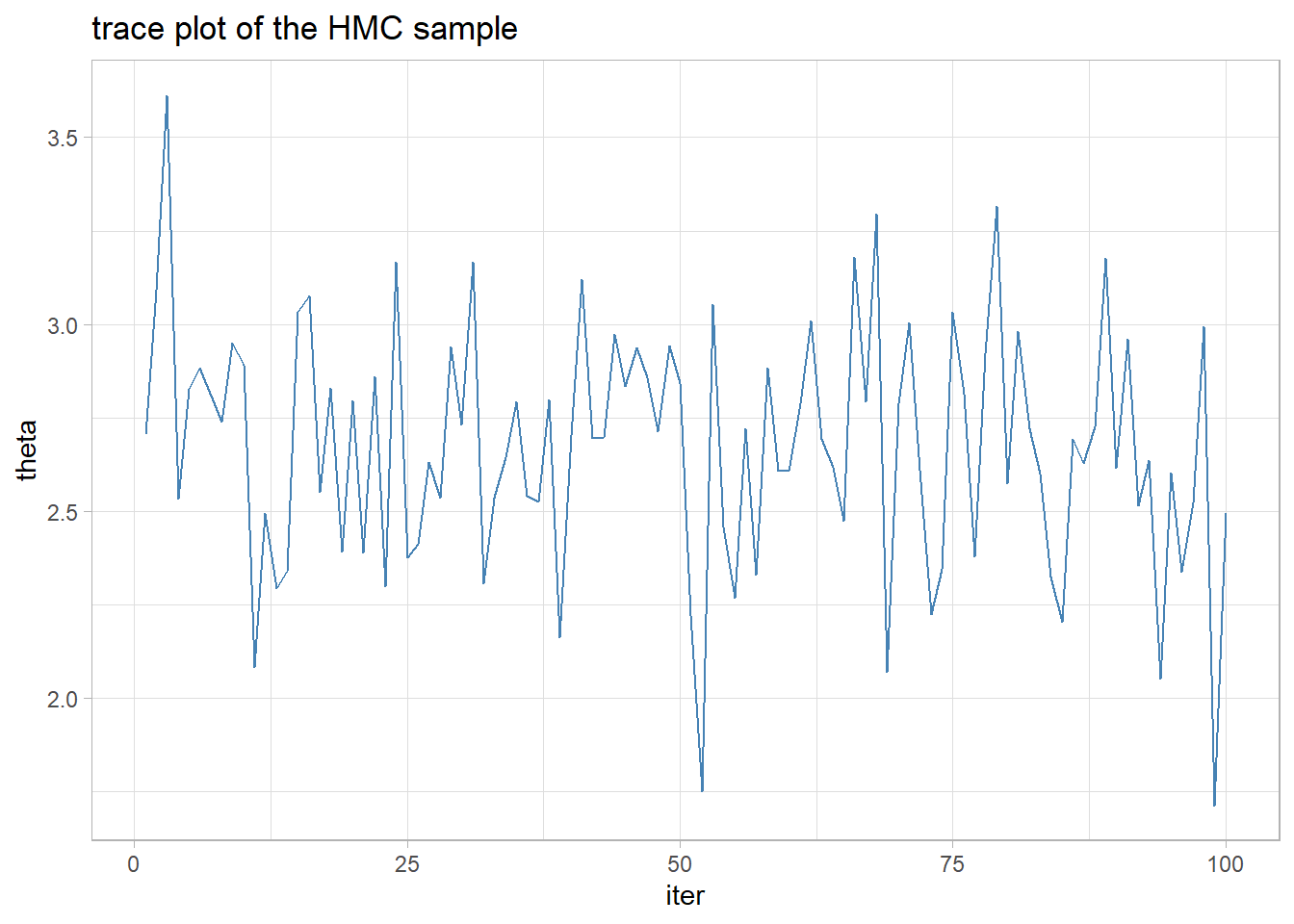
# --- histogram of the HMC sample ----------------------------
tibble( theta = sample ) %>%
  ggplot( aes(x=theta)) +
  geom_histogram( fill="steelblue", bins=25) +
  labs(title="Histogram of the HMC sample")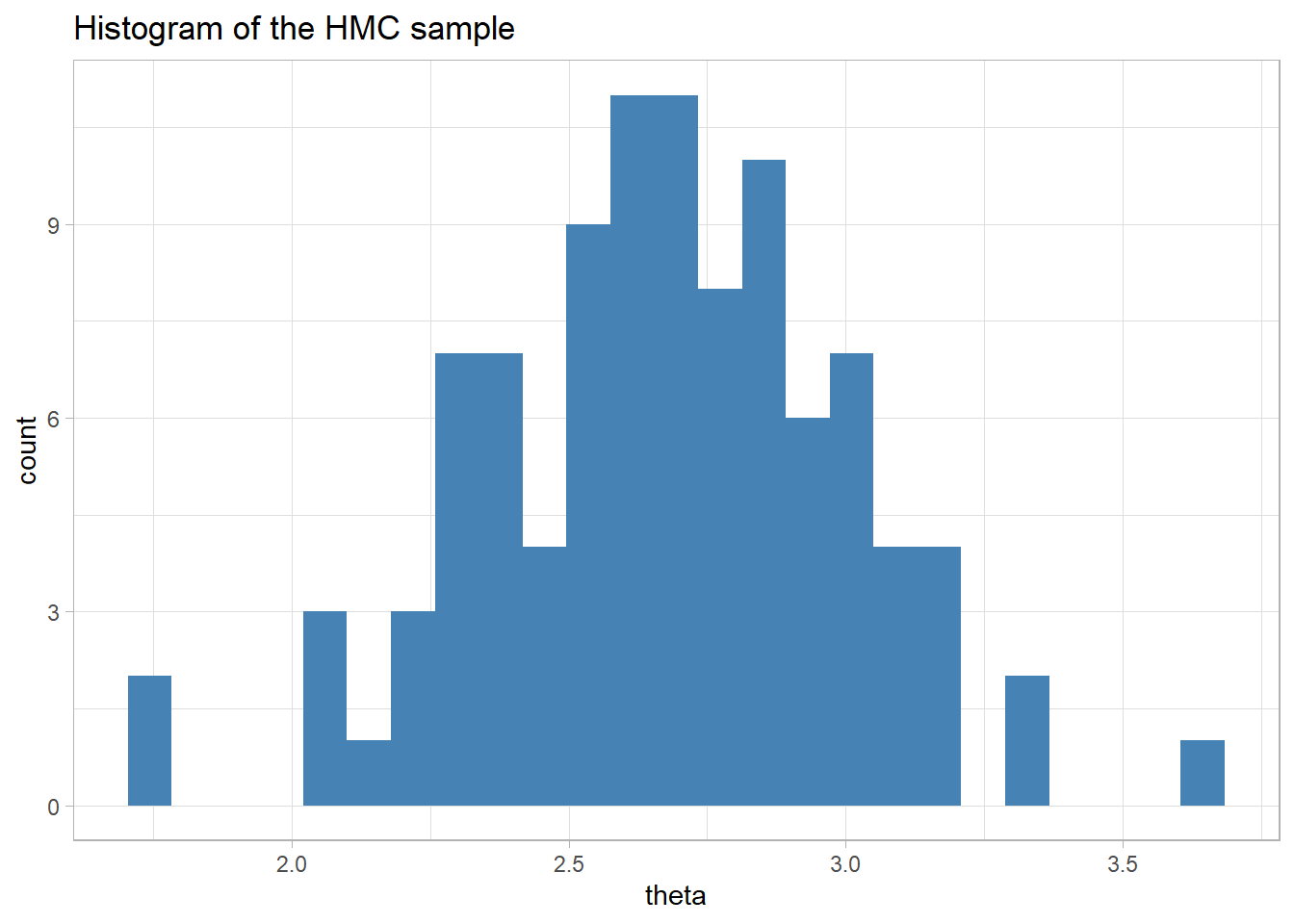
The mean of the sample is close to the mean of the data, as we would expect it to be when the prior is flat.
# --- posterior mean ------------
mean(sample)
## [1] 2.673291Not bad considering that I guessed at the time interval and the number of leap-frog steps, my initial value for theta was poorly chosen and I only ran 100 iterations.
Here is the histogram of the sample when 5000 iterations are run. Everything else remains unchanged.
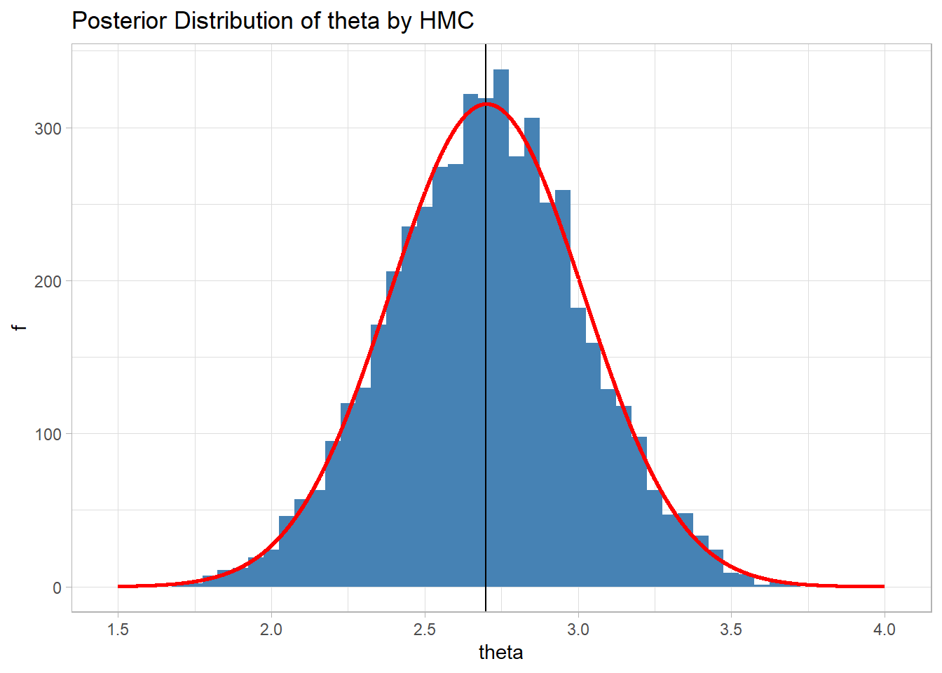
The estimate of the posterior mean is now 2.70 and the sample gives a good representation of the theoretical posterior that I have shown in red.