Sliced Episode 12: Loan Defaults
Summary
Background: In the final (episode 12) of the 2021 series of Sliced, the competitors were given two hours in which to analyse a set of data on bank loans. The aim was to predict the size of the default on the loan (usually zero). The metric for evaluation was the mean absolute error.
My approach: I explored the data and decided to build two models, one to predict whether or not the customer would default and the other to predict the size of the default in customers who defaulted. The size of the default is obviously related to the amount loaned, so for the second model I predicted the proportion of the loan that was defaulted. Both models were fitted using xgboost.
Result: Predictions for the size of the default were taken from the second model, but were replaced by zero if the first model suggested that the customer would not default. The resulting predictions would have come top of the leaderboard by a relatively large margin.
Conclusion: In the previous two episodes I had experimented with mlr3, but for this analysis I reverted to dplyr plus base R code. I felt closer to the data and I think that this helped me to find the best model. The alternative approach of directly minimising mean absolute error in an automatic algorithm does not perform well.
Introduction
The data for the final of Sliced 2021 can be downloaded from www.kaggle.com/c/sliced-s01e12-championship/overview. The organisers selected a set of data on business loans made by a bank and asked the finalists to predict the size of any default, evaluating the models by mean absolute error.
The choice of mean absolute error was an interesting one, not because it is particularly appropriate to the problem, but more because it moved the competitors out of their comfort zone.
Reading the data
It is my practice to read the data asis and to immediately save it in rds format within a directory called data/rData. For details of the way that I organise my analyses you should read my post called Sliced Methods Overview.
# --- setup: libraries & options ------------------------
library(tidyverse)

theme_set( theme_light())

# --- set home directory -------------------------------
home <- "C:/Projects/kaggle/sliced/s01-e12"

# --- read downloaded data -----------------------------
trainRawDF <- readRDS( file.path(home, "data/rData/train.rds") )

testRawDF <- readRDS( file.path(home, "data/rData/test.rds") )
Data Exploration
I usually start by summarising the training data with the skimr package and as always, I hide the output because of its length.
# --- summarise the training set -----------------------
skimr::skim(trainRawDF)
From skim() I learn that there are 83,656 loans and only 16 missing values, all for the variable NewExist, which measures whether the loan was to a new or an existing business.
The Response
The response is the default_amount, which I tabulate using kable.
library(kableExtra)

trainRawDF %>%
  mutate( default = factor(default_amount> 0,
                           levels=c(FALSE, TRUE),
                           labels=c("Repaid", "Defaulted"))) %>%
  group_by( default) %>%
  summarise( n      = n(),
             mean   = mean(default_amount),
             median = median(default_amount),
             min    = min(default_amount),
             max    = max(default_amount),
                      .groups="drop") %>%
  mutate( pct = round(100*n/sum(n),1) ) %>%
  select( default, n, pct, mean, median, min, max) %>%
  kable(caption="Amount defaulted") %>%
kable_classic(full_width=FALSE)| default | n | pct | mean | median | min | max |
|---|---|---|---|---|---|---|
| Repaid | 64457 | 77.1 | 0.00 | 0 | 0 | 0 |
| Defaulted | 19199 | 22.9 | 62879.67 | 27552 | 5 | 1895579 |
77% of loans are not defaulted, but defaults can be up be anything from $5 to $1.9 million
Here is a histogram of the non-zero defaults.
# --- non-zero defaults ----------------------------
trainRawDF %>%
  filter( default_amount > 0 ) %>%
  ggplot( aes(x=default_amount)) +
  geom_histogram( bins=100, fill="steelblue") +
  labs(x = "Amount defaulted",
       title = "Size of default when loan not repaid")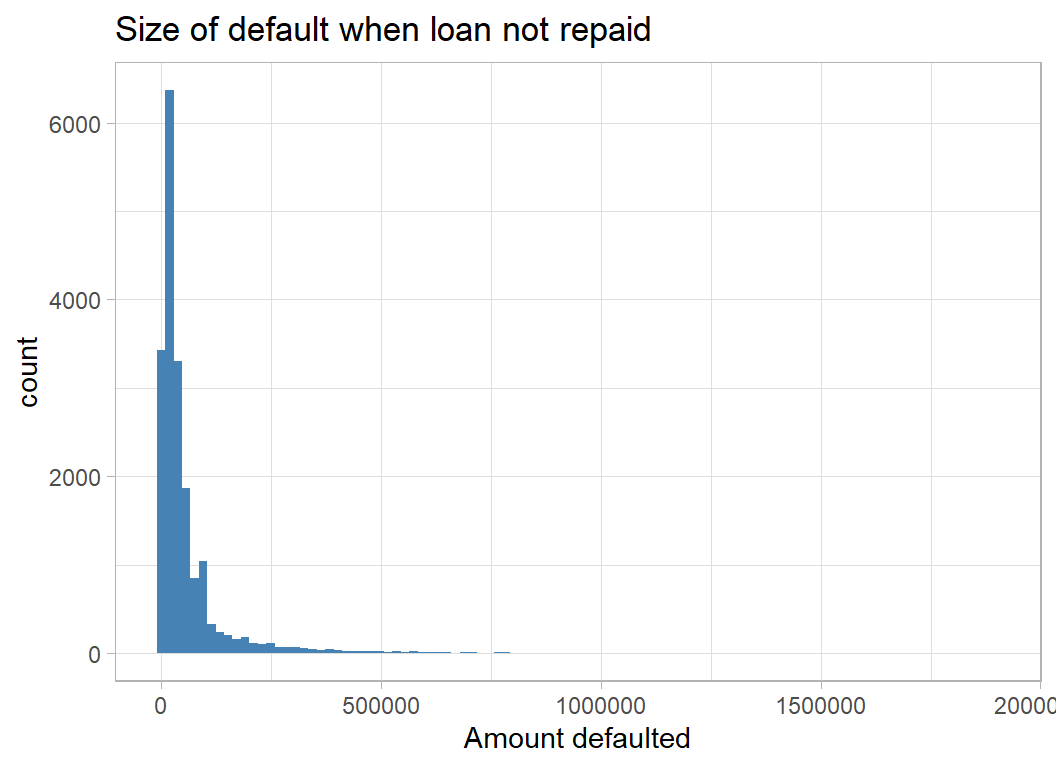
The amounts defaulted are very skew, so they are better viewed on a log scale
# --- log10 non-zero defaults ----------------------
trainRawDF %>%
  filter( default_amount > 0 ) %>%
  ggplot( aes(x=log10(default_amount))) +
  geom_histogram( bins=100, fill="steelblue") +
  labs(x = "log10(Amount defaulted)",
       title = "Size of default when loan not repaid")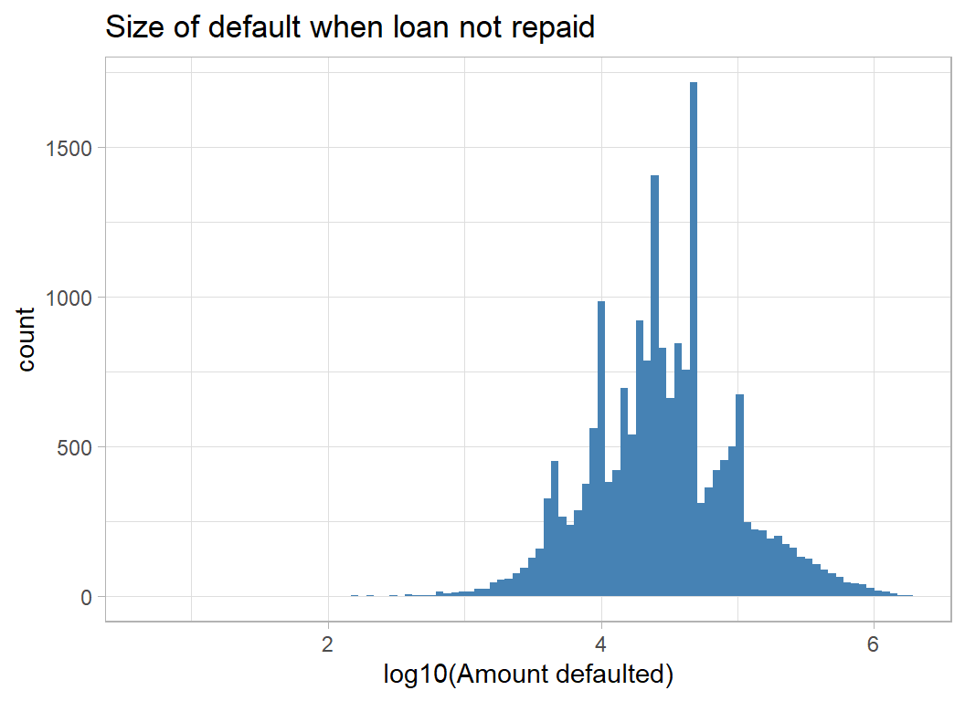
The Predictors
I consider each of the predictors starting with the business sector.
Sector
The rate of defaulting varies by business sector, from about 10% in Agriculture and Management to a rate that is 3 times higher in Finance and Real Estate.
trainRawDF %>%
  mutate( default = factor(default_amount> 0,
                           levels=c(FALSE, TRUE),
                           labels=c("repaid", "default"))) %>%
  group_by(Sector, default) %>%
  summarise( n = n(), .groups="drop") %>%
  pivot_wider( values_from=n, names_from=default) %>%
  mutate( pct = 100*default/(default+repaid))
## # A tibble: 20 x 4
## Sector repaid default pct
## <chr> <int> <int> <dbl>
## 1 Accommodation and food services 5865 1878 24.3
## 2 Administrative and support and waste management and rem~ 2904 1103 27.5
## 3 Agriculture, forestry, fishing and hunting 788 86 9.84
## 4 Arts, entertainment, and recreation 1291 389 23.2
## 5 Construction 5892 2142 26.7
## 6 Educational services 612 232 27.5
## 7 Finance and insurance 837 395 32.1
## 8 Health care and social assistance 5869 759 11.5
## 9 Information 1031 396 27.8
## 10 Management of companies and enterprises 27 3 10
## 11 Manufacturing 6386 1318 17.1
## 12 Mining, quarrying, and oil and gas extraction 147 20 12.0
## 13 Other services (except public administration) 6954 1970 22.1
## 14 Professional, scientific, and technical services 6805 1874 21.6
## 15 Public administration 26 5 16.1
## 16 Real estate and rental and leasing 1128 578 33.9
## 17 Retail trade 11553 3853 25.0
## 18 Transportation and warehousing 1791 873 32.8
## 19 Utilities 60 9 13.0
## 20 Wholesale trade 4491 1316 22.7NAICS
North American Industry Classification System (NAICS) is a numerical system for coding industries. The full code has 6 digits, but the first 2 digits are often used for a less detailed breakdown. The first two digits correspond very closely to Sector, the feature that I have just looked at.
As an example, I take NAICS 541940. 54 refers to all “Professional, Scientific, and Technical Services” and 541940 refers to “Vets”
You can check the codes at www.census.gov/naics
Here are the 6 digit codes with the highest and lowest default rates.
# --- NAICS industry classification -----------------------
#
options(knitr.kable.NA = '..')

trainRawDF %>%
  mutate( default = factor(default_amount> 0,
                           levels=c(FALSE, TRUE),
                           labels=c("repaid", "defaulted"))) %>%
  group_by(NAICS, default) %>%
  summarise( n = n(), .groups="drop") %>%
  pivot_wider( values_from=n, names_from=default, values_fill=0 ) %>%
  mutate( Percent = round(100*defaulted/(defaulted+repaid),1)) %>%
  # --- at least 50 loans in this sector ------------------
  filter( repaid + defaulted > 50) %>%
  # --- top and bottom 3 ----------------------------------
  arrange( Percent ) %>%
  filter(row_number() > max(row_number()) - 3 |
           row_number() <= 3) %>%
  add_row( Percent = 20)  %>%
  arrange( Percent) %>%
  mutate( Percent = ifelse(Percent == 20, NA, Percent)) %>%
  kable(caption="NAICS codes with the highest and lowest default rates") %>%
kable_classic(full_width=FALSE) | NAICS | repaid | defaulted | Percent |
|---|---|---|---|
| 514210 | 54 | 1 | 1.8 |
| 421830 | 211 | 6 | 2.8 |
| 421930 | 66 | 2 | 2.9 |
| .. | .. | .. | .. |
| 522310 | 127 | 157 | 55.3 |
| 488999 | 39 | 52 | 57.1 |
| 236116 | 37 | 53 | 58.9 |
51 is the information sector and 23 is construction.
Location
You can look separately at the State of the loanee and the State of the bank. The ranges of default rates are surprising to me, but this is probably a reflection of not living in the USA.
The key message seems to be, don’t loan to businesses based in Florida
# --- state of loanee --------------------------------
# --- top 3 and bottom 3 rates -----------------------
trainRawDF %>%
  mutate( default = factor(default_amount> 0,
                           levels=c(FALSE, TRUE),
                           labels=c("repaid", "default"))) %>%
  group_by(State, default) %>%
  summarise( n = n(), .groups="drop") %>%
  pivot_wider( values_from=n, names_from=default, values_fill=0 ) %>%
  mutate( Percent = round(100*default/(default+repaid),1)) %>%
  # --- at least 50 loans in this sector ------------------
  filter( repaid + default > 50) %>%
  # --- top and bottom 3 ----------------------------------
  arrange( Percent ) %>%
  filter(row_number() > max(row_number()) - 3 |
           row_number() <= 3) %>%
  add_row( Percent = 20)  %>%
  arrange( Percent) %>%
  mutate( Percent = ifelse(Percent == 20, NA, Percent)) %>%
  kable(caption="Home State of the Loanee") %>%
kable_classic(full_width=FALSE) | State | repaid | default | Percent |
|---|---|---|---|
| ND | 204 | 10 | 4.7 |
| MT | 541 | 46 | 7.8 |
| WY | 137 | 12 | 8.1 |
| .. | .. | .. | .. |
| GA | 1340 | 649 | 32.6 |
| DC | 121 | 60 | 33.1 |
| FL | 2869 | 1573 | 35.4 |
Don’t borrow from a bank in Virginia (unless plan to default).
# --- state of  Bank --------------------------------
# --- top 3 and bottom 3 rates -----------------------
trainRawDF %>%
  mutate( default = factor(default_amount> 0,
                           levels=c(FALSE, TRUE),
                           labels=c("repaid", "default"))) %>%
  group_by(BankState, default) %>%
  summarise( n = n(), .groups="drop") %>%
  pivot_wider( values_from=n, names_from=default, values_fill=0 ) %>%
  mutate( Percent = round(100*default/(default+repaid),1)) %>%
  # --- at least 50 loans in this sector ------------------
  filter( repaid + default > 50) %>%
  # --- top and bottom 3 ----------------------------------
  arrange( Percent ) %>%
  filter(row_number() > max(row_number()) - 3 |
           row_number() <= 3) %>%
  add_row( Percent = 20)  %>%
  arrange( Percent) %>%
  mutate( Percent = ifelse(Percent == 20, NA, Percent)) %>%
  kable(caption="Home State of the Bank") %>%
kable_classic(full_width=FALSE) | BankState | repaid | default | Percent |
|---|---|---|---|
| ME | 163 | 4 | 2.4 |
| DC | 197 | 6 | 3.0 |
| AZ | 300 | 11 | 3.5 |
| .. | .. | .. | .. |
| DE | 2268 | 900 | 28.4 |
| NC | 6841 | 3447 | 33.5 |
| VA | 2123 | 1663 | 43.9 |
An interesting feature is whether the business borrowed from a local bank, by which I mean a bank in its own state.
# --- local (in-state) loans ------------------------------
trainRawDF %>%
  mutate( default = factor(default_amount> 0,
                           levels=c(FALSE, TRUE),
                           labels=c("repaid", "default"))) %>%
  mutate( inState = factor(State == BankState,
                           levels=c(FALSE, TRUE),
                           labels=c("No", "Yes"))) %>%
  group_by(inState, default) %>%
  summarise( n = n(), .groups="drop") %>%
  pivot_wider( values_from=n, names_from=default, values_fill=0 ) %>%
  mutate( pct = 100*default/(default+repaid)) %>%
  arrange( pct )
## # A tibble: 2 x 4
## inState repaid default pct
## <fct> <int> <int> <dbl>
## 1 Yes 28827 3961 12.1
## 2 No 35630 15238 30.0Borrowing out of state is more common and is more likely to result in a default.
Urban/Rural
We also know whether the company is urban or rural.
# --- urban=1 or rural=2 or undefined=0 ----------------
trainRawDF %>%
  mutate( default = factor(default_amount> 0,
                           levels=c(FALSE, TRUE),
                           labels=c("repaid", "default"))) %>%
  mutate( UrbanRural = factor(UrbanRural,
                           levels=0:2,
                           labels=c("Undefined", "Urban", "Rural"))) %>%
  group_by(UrbanRural, default) %>%
  summarise( n = n(), .groups="drop") %>%
  pivot_wider( values_from=n, names_from=default, values_fill=0 ) %>%
  mutate( pct = 100*default/(default+repaid)) %>%
  arrange( pct )
## # A tibble: 3 x 4
## UrbanRural repaid default pct
## <fct> <int> <int> <dbl>
## 1 Undefined 15196 998 6.16
## 2 Rural 7951 2288 22.3
## 3 Urban 41310 15913 27.8Bank
There are over 300 different banks. Here are the top 5 and the bottom 5 for defaults.
# --- state of  Bank --------------------------------
trainRawDF %>%
  mutate( default = factor(default_amount> 0,
                           levels=c(FALSE, TRUE),
                           labels=c("repaid", "default"))) %>%
  group_by(Bank, default) %>%
  summarise( n = n(), .groups="drop") %>%
  pivot_wider( values_from=n, names_from=default, values_fill=0 ) %>%
  mutate( Percent = round(100*default/(default+repaid),1)) %>%
  # --- at least 50 loans in this sector ------------------
  filter( repaid + default > 50) %>%
  # --- top and bottom 3 ----------------------------------
  arrange( Percent ) %>%
  filter(row_number() > max(row_number()) - 5 |
           row_number() <= 5) %>%
  add_row( Percent = 20)  %>%
  arrange( Percent) %>%
  mutate( Percent = ifelse(Percent == 20, NA, Percent)) %>%
  kable(caption="Best and Worst Banks") %>%
kable_classic(full_width=FALSE) | Bank | repaid | default | Percent |
|---|---|---|---|
| BAY AREA EMPLOYMENT DEVEL CO | 73 | 0 | 0.0 |
| BUSINESS DEVEL FINAN CORP | 108 | 0 | 0.0 |
| BUSINESS FINANCE GROUP, INC. | 97 | 0 | 0.0 |
| CALIFORNIA STATEWIDE CERT. DEV | 124 | 0 | 0.0 |
| CAPITAL ACCESS GROUP, INC. | 58 | 0 | 0.0 |
| .. | .. | .. | .. |
| HSBC BK USA NATL ASSOC | 343 | 264 | 43.5 |
| BANCO POPULAR NORTH AMERICA | 499 | 461 | 48.0 |
| BBCN BANK | 1294 | 2092 | 61.8 |
| SUPERIOR FINANCIAL GROUP, LLC | 162 | 473 | 74.5 |
| CAPITAL ONE BK (USA) NATL ASSO | 8 | 53 | 86.9 |
Some of these rates are so poor that it is hard to credit. How can they still be in business? The data comes from the years 1990-2010 so perhaps these data reflect the impact of the 2008 financial crisis. Even so!
Year of Loan
The plot of default rate by financial year confirms the importance of the 2007-2008 crisis. It is interesting that these data make it look as though the financial crisis was predictable in 2005.
trainRawDF %>%
  mutate( default = factor(default_amount> 0,
                           levels=c(FALSE, TRUE),
                           labels=c("repaid", "default"))) %>%
  group_by(ApprovalFY, default) %>%
  summarise( n = n(), .groups="drop") %>%
  pivot_wider( values_from=n, names_from=default, values_fill=0 ) %>%
  mutate( pct = 100*default/(default+repaid)) %>%
  arrange( pct ) %>%
  ggplot( aes(x=ApprovalFY, y=pct)) +
  geom_line() +
  labs( x= "Year loan approaved",
        y = "Percent defaulting",
        title = "Pattern of defaults over time")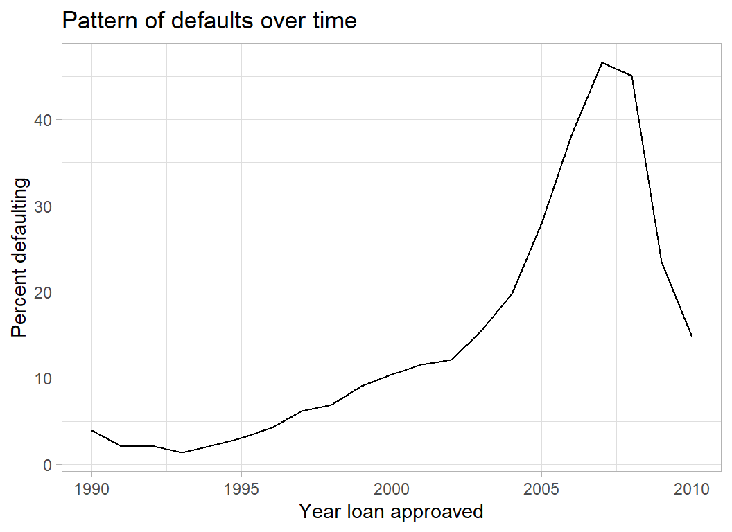
New and Existing Businesses
The coding is, 1 for an existing business and 2 for a new business. There are 16 missing codes and 60 businesses coded as 0. Zero codes are not mentioned in the data dictionary.
trainRawDF %>%
  mutate( default = factor(default_amount> 0,
                           levels=c(FALSE, TRUE),
                           labels=c("repaid", "default"))) %>%
  mutate( NewExist = factor(NewExist),
          NewExist = fct_explicit_na(NewExist)) %>%
  group_by(NewExist, default) %>%
  summarise( n = n(), .groups="drop") %>%
  pivot_wider( values_from=n, names_from=default, values_fill=0 ) %>%
  mutate( pct = 100*default/(default+repaid)) %>%
  arrange( pct )
## # A tibble: 4 x 4
## NewExist repaid default pct
## <fct> <int> <int> <dbl>
## 1 0 56 4 6.67
## 2 (Missing) 14 2 12.5
## 3 1 47694 13951 22.6
## 4 2 16693 5242 23.9I think that it would make sense to merge missing and zero.
Size of the Company
Companies with many employees are less likely to default.
# --- number of employees -----------------------
trainRawDF %>%
  mutate( default = factor(default_amount> 0,
                           levels=c(FALSE, TRUE),
                           labels=c("repaid", "default"))) %>%
  mutate( NoEmp = cut(NoEmp, breaks=c(0, 1, 5, 10, 100, 10000 ), include.lowest=TRUE, dig.lab=5)) %>%
  group_by(NoEmp, default) %>%
  summarise( n = n(), .groups="drop") %>%
  pivot_wider( values_from=n, names_from=default, values_fill=0 ) %>%
  mutate( pct = 100*default/(default+repaid))
## # A tibble: 5 x 4
## NoEmp repaid default pct
## <fct> <int> <int> <dbl>
## 1 [0,1] 12372 5032 28.9
## 2 (1,5] 26738 9110 25.4
## 3 (5,10] 11087 2908 20.8
## 4 (10,100] 13813 2124 13.3
## 5 (100,10000] 447 25 5.30CreateJob measures the number of new jobs created by the loan. When the number is large the default rate is lower. Of course, this factor will not be independent of the original size of the company.
trainRawDF %>%
  mutate( default = factor(default_amount> 0,
                           levels=c(FALSE, TRUE),
                           labels=c("repaid", "default"))) %>%
  mutate( CreateJob = cut(CreateJob, breaks=c(0, 1, 5, 10, 2000 ), include.lowest=TRUE, dig.lab=4)) %>%
  group_by(CreateJob, default) %>%
  summarise( n = n(), .groups="drop") %>%
  pivot_wider( values_from=n, names_from=default, values_fill=0 ) %>%
  mutate( pct = 100*default/(default+repaid))
## # A tibble: 4 x 4
## CreateJob repaid default pct
## <fct> <int> <int> <dbl>
## 1 [0,1] 48165 13758 22.2
## 2 (1,5] 10391 4166 28.6
## 3 (5,10] 3048 764 20.0
## 4 (10,2000] 2853 511 15.2Loans that help companies retain jobs are more likely to be repaid.
trainRawDF %>%
  mutate( default = factor(default_amount> 0,
                           levels=c(FALSE, TRUE),
                           labels=c("repaid", "default"))) %>%
  mutate( RetainedJob = cut(RetainedJob,
                            breaks=c(0, 1, 5, 10, 100, 5000 ),
                            include.lowest=TRUE, dig.lab=4)) %>%
  group_by(RetainedJob, default) %>%
  summarise( n = n(), .groups="drop") %>%
  pivot_wider( values_from=n, names_from=default, values_fill=0 ) %>%
  mutate( pct = 100*default/(default+repaid))
## # A tibble: 5 x 4
## RetainedJob repaid default pct
## <fct> <int> <int> <dbl>
## 1 [0,1] 32486 6760 17.2
## 2 (1,5] 17317 7885 31.3
## 3 (5,10] 7001 2635 27.3
## 4 (10,100] 7463 1899 20.3
## 5 (100,5000] 190 20 9.52Franchise
The Franchise code is undefined in the data dictionary. We are told that 0 and 1 correspond to businesses that are not franchises. So I’ll just consider Franchise Yes/No.
trainRawDF %>%
  mutate( default = factor(default_amount> 0,
                           levels=c(FALSE, TRUE),
                           labels=c("repaid", "default"))) %>%
  mutate( Franchise = factor(FranchiseCode > 1,
                           levels=c(FALSE, TRUE),
                           labels=c("No", "Yes"))) %>%
  group_by(Franchise, default) %>%
  summarise( n = n(), .groups="drop") %>%
  pivot_wider( values_from=n, names_from=default, values_fill=0 ) %>%
  mutate( pct = 100*default/(default+repaid)) %>%
  arrange( pct )
## # A tibble: 2 x 4
## Franchise repaid default pct
## <fct> <int> <int> <dbl>
## 1 Yes 3201 809 20.2
## 2 No 61256 18390 23.1So franchises are the minority and they are slightly less likely to default.
Size of the loan
Disbursement refers to the amount loaned.
trainRawDF %>%
  mutate( default = factor(default_amount> 0,
                           levels=c(FALSE, TRUE),
                           labels=c("repaid", "default"))) %>%
  mutate( Disbursement = cut(DisbursementGross,
      breaks=c(0, quantile(DisbursementGross,
                           probs=seq(0.1, 1.0, by=0.1))),
      dig.lab=7)) %>%
  group_by(Disbursement, default) %>%
  summarise( n = n(), .groups="drop") %>%
  pivot_wider( values_from=n, names_from=default, values_fill=0 ) %>%
  mutate( pct = 100*default/(default+repaid)) %>%
  arrange( pct )
## # A tibble: 10 x 4
## Disbursement repaid default pct
## <fct> <int> <int> <dbl>
## 1 (480659,5294366] 7638 728 8.70
## 2 (255000,480659] 7380 944 11.3
## 3 (157108,255000] 7014 1393 16.6
## 4 (110000,157108] 6632 1677 20.2
## 5 (80000,110000] 6408 2007 23.9
## 6 (54472,80000] 6254 2118 25.3
## 7 (25000,41211.5] 6101 2172 26.3
## 8 (41211.5,54472] 5866 2500 29.9
## 9 (15000,25000] 5343 2351 30.6
## 10 (0,15000] 5821 3309 36.2Businesses are more likely to default if the loan is small. Presumably, banks are less risk adverse when the amount is small.
When companies do default the size of the default is linked to the size of the loan
trainRawDF %>%
  filter( default_amount> 0) %>%
  ggplot( aes(x=DisbursementGross, y=default_amount) ) +
  geom_point() +
  geom_abline() +
  geom_smooth() +
  labs( x = "Size of the loan (disbursement)",
        y = "Size of the default",
        title = "Amount defaulted and the size of the loan")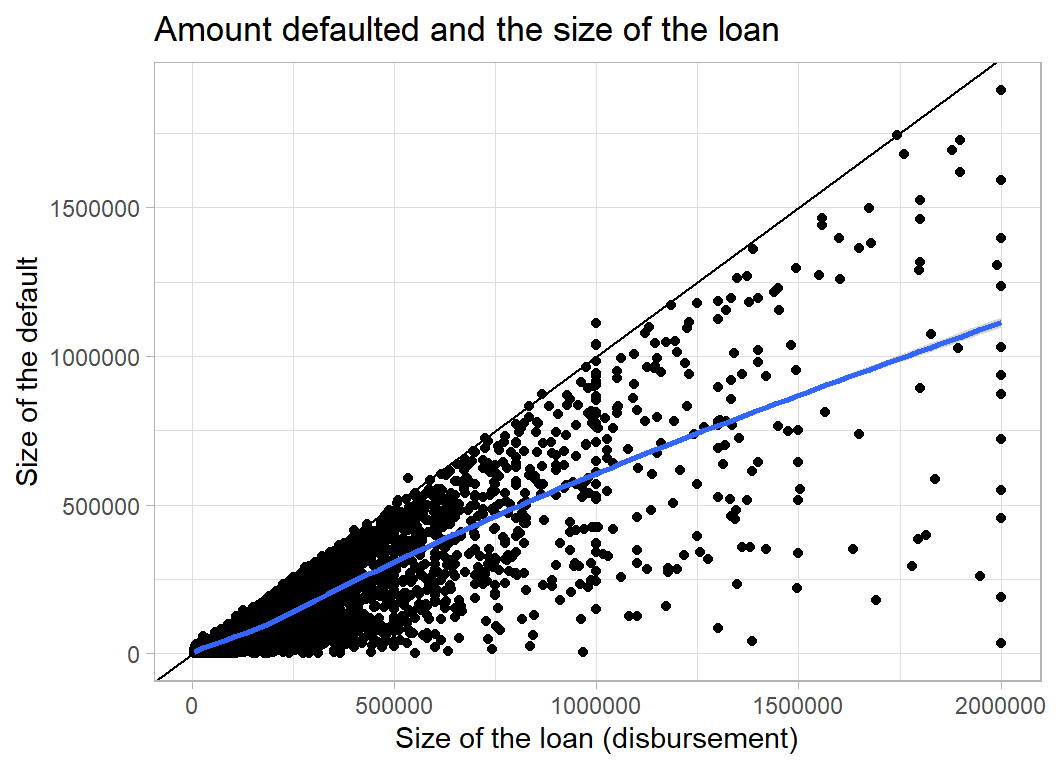
Alternatively, we can look at the percentage of the loan that is defaulted. Presumably the numbers over 100% refer to businesses that run up interest that they do not repay. On average, companies default on about 60% of the loan.
trainRawDF %>%
  filter( default_amount> 0) %>%
  ggplot( aes(x=DisbursementGross, y=100*default_amount/DisbursementGross) ) +
  geom_point() +
  geom_smooth() +
    labs( x = "Size of the loan (disbursment)",
        y = "Percent of loan defaulted",
        title = "Percent defaulted and the size of the loan")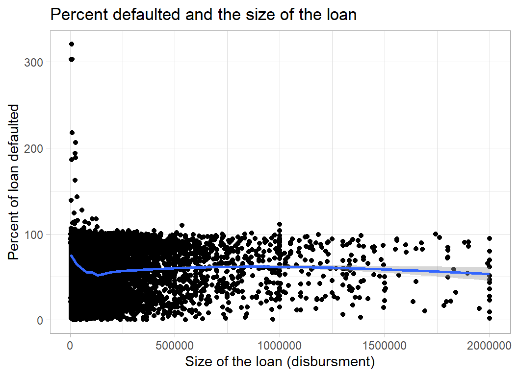
GrAppv measures the amount that the bank originally approved. In most cases it is very similar to the Disbursement.
trainRawDF %>%
  ggplot( aes(x=GrAppv/100000, y=DisbursementGross/100000) ) +
  geom_point() +
  geom_abline()  +
    labs( y = "Size of the loan (disbursment)",
        x = "Amount originally approved",
        title = "Amount approved and amount eventually loaned in units of $100,000")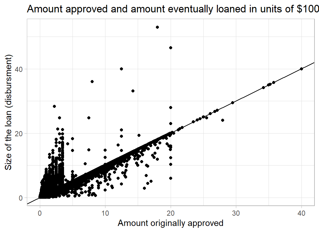
SBA_Appv is the amount guaranteed by the SBA (Small Business Administration), an organisation created to help small businesses
trainRawDF %>%
  filter( SBA_Appv > 0 ) %>%
  ggplot( aes(y=SBA_Appv/100000, x=GrAppv/100000) ) +
  geom_point() +
  geom_abline() +
  labs( y = "SBA Guarantee ($100,000)",
        x = "Amount Approved ($100,000)",
        title = "SBA Guarantees")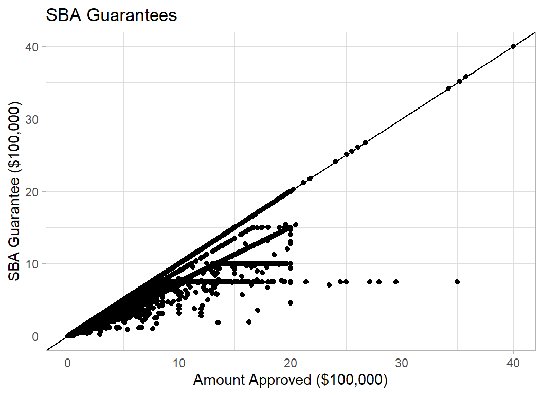
Data Cleaning
There are multiple codes for Bank, State, BankState and NAICS, so I have decided to use three digits of NAICS and to lump the smaller categories into an ‘Other’ category.
I have also decided to drop Sector as it duplicates NAICS and to ignore Zip code and City. Name is the name of the business and I’ve dropped that as well.
trainRawDF %>%
   mutate( NewExist = factor(ifelse( is.na(NewExist),
                                     0, NewExist)),
           inState  = as.numeric( State == BankState),
           Bank     = factor(Bank),
           Bank     = fct_lump_prop(Bank, prop=0.001),
           State    = factor(State),
           State    = fct_lump_prop(State, prop=0.01),
           BankState = factor(BankState),
           BankState = fct_lump_prop(BankState, prop=0.01),
           FranchiseCode = ifelse( FranchiseCode <= 1, 0, 1),
           UrbanRural = factor(UrbanRural),
           NAICS      = factor(floor(NAICS/1000)),
           NAICS     = fct_lump_prop(NAICS, prop=0.001)) %>%
  select( -LoanNr_ChkDgt, -Name, -Sector, -City, -Zip ) -> trainDF
The test data must be coded in the same way. That is, I must use the levels of the training data after lumping and not lump the test data.
testRawDF %>%
   mutate( NewExist = factor(ifelse( is.na(NewExist), 0, NewExist)),
           inState  = as.numeric( State == BankState),
           Bank     = factor(Bank,
                             levels=levels(trainDF$Bank)),
           Bank     = fct_explicit_na(Bank, na_level="Other"),
           State    = factor(State,
                             levels=levels(trainDF$State)),
           State    = fct_explicit_na(State, na_level="Other"),
           BankState     = factor(BankState,
                             levels=levels(trainDF$BankState)),
           BankState     = fct_explicit_na(BankState,
                                           na_level="Other"),
           FranchiseCode = ifelse( FranchiseCode <= 1, 0, 1),
           UrbanRural = factor(UrbanRural),
           NAICS      = factor(floor(NAICS/1000),
                               levels=levels(trainDF$NAICS)),
           NAICS     = fct_explicit_na(NAICS,
                                           na_level="Other") ) %>%
  select( -Name, -Sector, -City, -Zip ) -> testDF
I plan to use xgboost so I need to convert the factors into indicators, I’ll do that with my add_dummy() functions (see Appendix)
# --- Add indicators to training set ------------------------
trainDF %>%
  add_dummy( Bank, "B") %>%
  add_dummy( State, "S") %>%
  add_dummy( UrbanRural, "U") %>%
  add_dummy( NewExist, "E") %>%
  add_dummy( NAICS, "N") %>%
  add_dummy( BankState, "T") %>%
  select( -Bank, -State, -BankState, -UrbanRural,
          -NewExist, -NAICS) -> trainDF

# --- Add indicators to test set ----------------------------
testDF %>%
  add_dummy( Bank, "B") %>%
  add_dummy( State, "S") %>%
  add_dummy( UrbanRural, "U") %>%
  add_dummy( NewExist, "E") %>%
  add_dummy( NAICS, "N") %>%
  add_dummy( BankState, "T") %>%
  select( -Bank, -State, -BankState, -UrbanRural,
          -NewExist, -NAICS) -> testDF
Model Building
I want to create two models, one for the probability of defaulting and the other for the amount defaulted when companies do default.
I’ll create an estimation and validation set so that I can assess performance.
# --- Split into estimation and validation --------------
set.seed(7028)
split <- sample(1:83656, size=20000, replace=FALSE)

estimateDF <- trainDF[-split, ]
validateDF <- trainDF[ split, ]
Probability of a Default
First save the features and response in a matrix and vector.
library(xgboost)

# --- Estimation data to matrices ------------------------
estimateDF %>%
  select( -default_amount) %>%
  as.matrix() -> X

estimateDF %>%
  mutate(y = as.numeric(default_amount>0)) %>%
  pull(y) -> Y

dtrain <- xgb.DMatrix(data = X, label = Y)

# --- Validation data to matrices ------------------------
validateDF %>%
  select( -default_amount) %>%
  as.matrix() -> XV

validateDF %>%
  mutate(y = as.numeric(default_amount>0)) %>%
  pull(y) -> YV

dtest <- xgb.DMatrix(data = XV, label=YV)
Next I’ll investigate how many rounds are needed by fitting an xgboost model with what I hope is too many rounds.
# --- fit the xgboost model -----------------------------
xgb.train(data=dtrain,
        watchlist=list(train=dtrain, test=dtest),
        objective="binary:logistic",
        nrounds=200, verbose=0) -> xgmod
We can picture the performance as I did for the airbnb analysis.
# --- function to show train & validation metrics -------
xgmod$evaluation_log %>%
    ggplot( aes(x=iter, y=train_error)) +
    geom_line(colour="blue") +
    geom_line( aes(y=test_error), colour="red") +
    labs(x="Iteration", y="loss",
         title="In-sample and out-of-sample loss")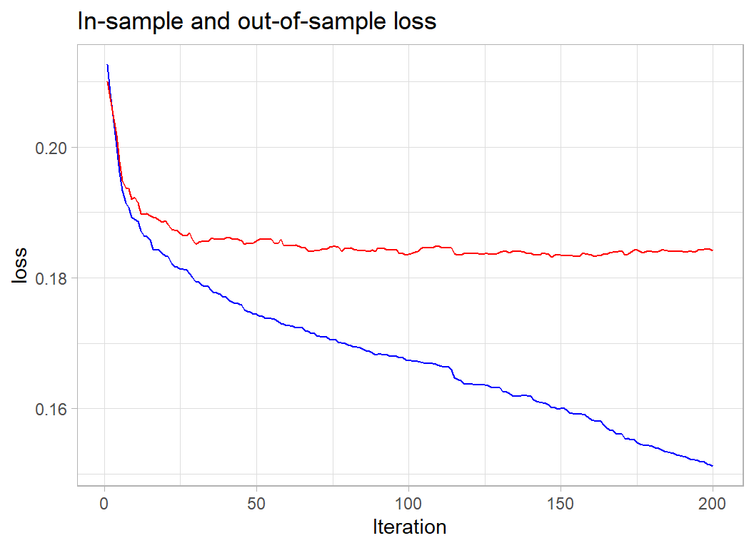
The 100 iterations looks reasonable. The loss here is the misclassification error, so we are misclassifying 18.5% of the businesses.
I’ll rerun with 100 rounds.
# --- fit the xgboost model -----------------------------
xgb.train(data=dtrain,
        watchlist=list(train=dtrain, test=dtest),
        objective="binary:logistic",
        nrounds=100, verbose=0) -> xgmod
and look at the predictions.
# --- Performance in the Validation set -----------------
validateDF %>%
  mutate( default = factor(default_amount> 0,
                           levels=c(FALSE, TRUE),
                           labels=c("repaid", "defaulted"))) %>%
  mutate( p = predict(xgmod, newdata=XV)) %>%
  mutate( predDefault = factor(p > 0.5,
                           levels=c(FALSE, TRUE),
                           labels=c("repaid", "defaulted"))) %>%
  group_by( default, predDefault)  %>%
  summarise( n = n(), .groups="drop")
## # A tibble: 4 x 3
## default predDefault n
## <fct> <fct> <int>
## 1 repaid repaid 14543
## 2 repaid defaulted 902
## 3 defaulted repaid 2771
## 4 defaulted defaulted 1784The model misclassifies 902 (6%) of those who actually repaid their loan and 2771 (61%) of those who default. Not that great.
Out of interest I look at the importance.
xgb.importance(model=xgmod) %>%
  as_tibble()
## # A tibble: 217 x 4
## Feature Gain Cover Frequency
## <chr> <dbl> <dbl> <dbl>
## 1 ApprovalFY 0.376 0.0754 0.104
## 2 SBA_Appv 0.105 0.0350 0.0860
## 3 DisbursementGross 0.0754 0.0299 0.148
## 4 B13 0.0524 0.0128 0.00773
## 5 inState 0.0387 0.0124 0.0145
## 6 GrAppv 0.0252 0.0143 0.0599
## 7 NoEmp 0.0219 0.0137 0.0705
## 8 CreateJob 0.0174 0.0175 0.0525
## 9 RetainedJob 0.0160 0.0138 0.0534
## 10 N64 0.0150 0.0140 0.00676
## # ... with 207 more rowsYear the loan approved is most important, reflecting the impact of the financial crisis.
Amount of the default
As before I extract the data into matrices. I will predict the proportion of the disbursement.
# --- Extract the Estimation data ---------------------
estimateDF %>%
  filter( default_amount > 0 ) %>%
  select( -default_amount) %>%
  as.matrix() -> X2

estimateDF %>%
  filter( default_amount > 0 ) %>%
  mutate( y = default_amount/DisbursementGross) %>%
  pull(y) -> Y2

dtrain <- xgb.DMatrix(data = X2, label = Y2)

# --- Extract the Validation data ---------------------
validateDF %>%
  filter( default_amount > 0 ) %>%
  select( -default_amount) %>%
  as.matrix() -> XV2

validateDF %>%
  filter( default_amount > 0 ) %>%
  mutate( y = default_amount/DisbursementGross) %>%
  pull(y) -> YV2

dtest <- xgb.DMatrix(data = XV2, label=YV2)
I’ll predict using xgboost with the mse criterion even though the final metric will be the mean absolute error.
First I investigate the number of rounds
# --- Model for proportion defaulted -----------------
xgb.train(data=dtrain,
        watchlist=list(train=dtrain, test=dtest),
         objective="reg:squarederror",
        nrounds=200, verbose=0) -> xgmod2

xgmod2$evaluation_log %>%
    ggplot( aes(x=iter, y=train_rmse)) +
    geom_line(colour="blue") +
    geom_line( aes(y=test_rmse), colour="red") +
    labs(x="Iteration", y="loss",
         title="In-sample and out-of-sample loss")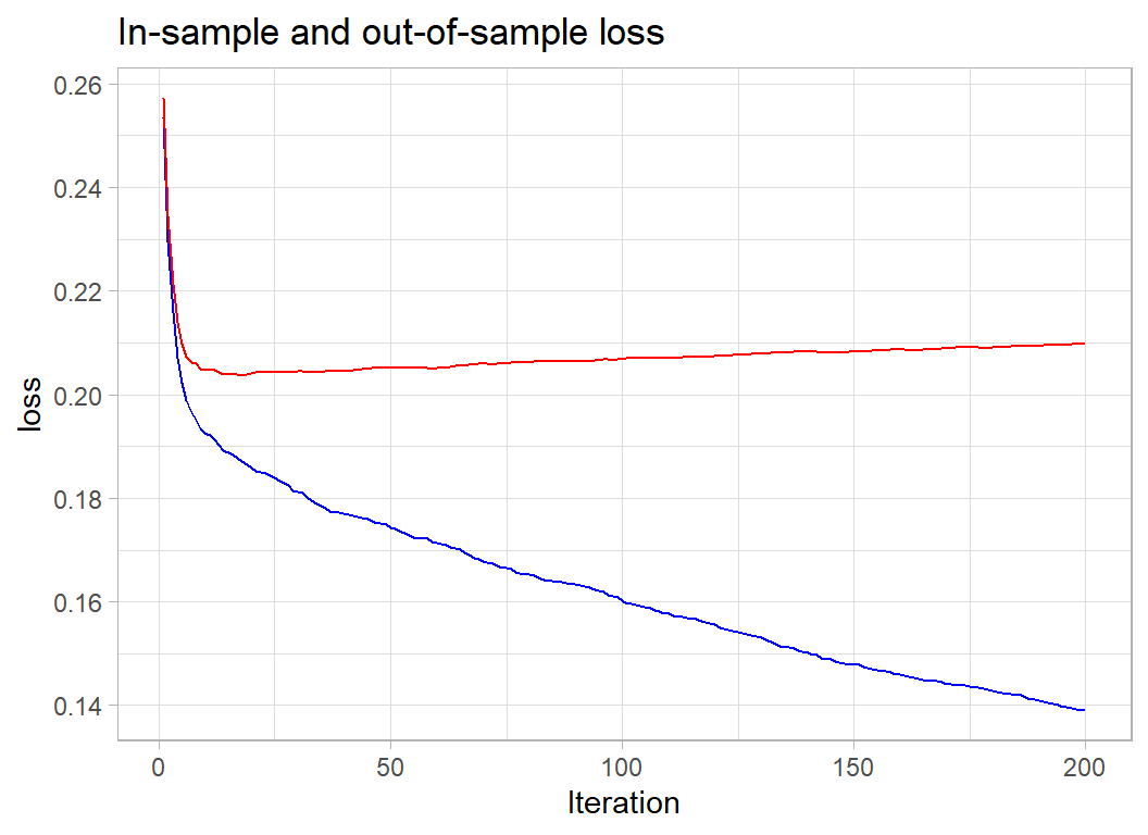
25 iterations would be enough.
# --- refit with 25 rounds --------------------------
xgb.train(data=dtrain,
        watchlist=list(train=dtrain, test=dtest),
         objective="reg:squarederror",
        nrounds=25, verbose=0) -> xgmod2
Prediction
I’ll predict for the full data set, making a prediction of the probability of default and of the amount. The final prediction will be zero if we predict no default and the predicted amount if we predict a default.
validateDF %>%
  mutate( p     = predict(xgmod, newdata=XV ) ) %>%
  mutate( yhat =  DisbursementGross*predict(xgmod2, newdata=XV )) %>%
  mutate( finalPrediction = (p>0.5)*yhat  ) %>%
  summarise( mean(abs(default_amount-finalPrediction)))
## # A tibble: 1 x 1
## `mean(abs(default_amount - finalPrediction))`
## <dbl>
## 1 13200.A mean absolute error (MAE) of 13,200. This promising because the leading model at the time of the competition scored 13,395 and David Robinson won the final with 13993.
Submission
I refit these models to the full training data.
# --- Probability of Default ---------------------

# --- Training data to matrices ------------------
trainDF %>%
  select( -default_amount) %>%
  as.matrix() -> X

trainDF %>%
  mutate(y = as.numeric(default_amount>0)) %>%
  pull(y) -> Y

dtrain <- xgb.DMatrix(data = X, label = Y)

# --- Model probability of default ---------------
xgb.train(data=dtrain,
         objective="binary:logistic",
        nrounds=100) -> xgmod

# --- Size of Default ----------------------------

# --- Training data to matrices ------------------
trainDF %>%
  filter( default_amount > 0 ) %>%
  select( -default_amount) %>%
  as.matrix() -> X

trainDF %>%
  filter( default_amount > 0 ) %>%
  mutate( y = default_amount/DisbursementGross) %>%
  pull(y) -> Y

dtrain <- xgb.DMatrix(data = X, label = Y)

# --- Model size of default ---------------------
xgb.train(data=dtrain,
         objective="reg:squarederror",
        nrounds=25) -> xgmod2
Now the predictions
# --- set the test data ---------------------------
testDF %>%
  select( -LoanNr_ChkDgt) %>%
  as.matrix() -> XT

# --- Make two-stage predictions ------------------
testDF %>%
  mutate( p     = predict(xgmod, newdata=XT ) ) %>%
  mutate( yhat =  DisbursementGross*predict(xgmod2, newdata=XT )) %>%
  mutate( default_amount = (p>0.5)*yhat  ) %>%
  select( LoanNr_ChkDgt, default_amount ) %>%
  write_csv( file.path(home, "temp/submission1.csv"))
13145 top!! without any tuning other than the number of iterations.
What I learned from this analysis
The main point to come out of this analysis is that the head-on approach of fitting a model that directly minimises the mean absolute error does not work well. I have not shown the results because the post is already too long, but I did try it as a secondary analysis. The dream of machine learning is that the data are fed into a giant algorithm that makes highly accurate predictions without any human input. This is just a dream and for the foreseeable future, it is likely to remain so. We are a long way from algorithms with the intelligence that would realise that the bank default problem could be split in two; whether there is a default and the proportion of the default.
The second thing that strikes me is the contrast between this analysis and an analysis based on a machine learning pipeline. In my previous two posts, I used mlr3, an ecosystem for organising machine learning projects and creating analysis pipelines. It is similar in its aim to tidymodels, although I think that mlr3 is better. This time, I reverted to my usual way of working and it felt like I had been set free. Having completed the analysis, I could now turn it into a pipeline, but I doubt if I would have produced such a successful analysis had I tried to develop it from scratch in mlr3 or tidymodels.
Of course, you would be justified in being a little wary of these opinions. I was trained as a statistician and it is hard to break with those traditions. I taught my students the importance of the analyst’s skill when developing a good model and so I cling to the idea that computers will never quite replace humans. History is against me.
Appendix
Function for creating indicator variables
add_dummy <- function(thisDF, col, prefix="X") {
  j <- 0
  sCol <- deparse(substitute(col))
  for( v in levels(thisDF[[sCol]])) {
    j <- j + 1
    dumName <- paste(prefix, j, sep="")
    thisDF[[dumName]] <- as.numeric(thisDF[[sCol]] == v )
  }
  return(thisDF)
}