Sliced Episode 1: Boardgame Ratings
Summary
Background: In episode 1 of the 2021 series of Sliced, the competitors were given two hours to analyse a set of data on boardgames. The aim was to predict the games’ ratings.
My approach: In the data exploration I transform the ratings and plot them against the potential predictors. I note inconsistencies in the data. The mechanics of the game and the type of game are described as text, so I create indicator variables for the words most closely associated with the games’ ratings. For my model, I use a spline-based generalised additive model (GAM) fitted with the package mgcv.
Result: A GAM based on selected predictors was comparable with other models towards the top of the Sliced leaderboard.
Conclusion: As well as producing good predictions, GAMs are interpretable and generalisable. After the analysis, I discuss the contrasting aims of modelling in statistics and machine learning.
Introduction
The data for the first episode of Sliced 2021 can be downloaded from https://www.kaggle.com/c/sliced-s01e01. The organisers took the data from https://boardgamegeek.com/, a site for all things associated with boardgames.
On the boardgamegeek (BGG) website, enthusiasts can rate the games that they play. The final geek rating is a value between 1 and 10 formed as a weighted combination of the average rating of the fans and 5.5 (the mid-point of the scale). The weighting that the site uses is not published, but it is chosen so that games with few user ratings are weighted more heavily towards 5.5 and games with many ‘votes’ are weighted towards the average fan rating. The method is intended to avoid games becoming highly rated based on very few votes.
The task for the contestants was to predict the geek rating from a range of predictors that describe different aspects of the game. There is a training set of 3,499 games and a test set of 1,500 games, which has the geek rating withheld. The Sliced site does not say explicitly what metric will be used to evaluate the predictions, but it fairly obvious that it is the root mean square error (RMSE).
On the Sliced website, there is a leaderboard that shows the performance of submissions made by the contestants and the viewers while the show was live. The people submitting were able to see a real time measure of performance on the public leaderboard, but this is based on only 1% of the test data. At the end of the show, the private leaderboard using the other 99% was revealed. Withholding the results for the bulk of the training data, both increases the tension in the show and it stops contestants from tuning their models towards good performance on the test set. Often the scores of the same model on the private and public leaderboards are very different.
The Sliced website is still live and anyone can make late submissions and discover how they would have scored, although they will not added to the leaderboard. When I report a submissions, I judge it by the more accurate, private leaderboard score.
My background as a biostatistician leads me to believe that, for this type of data, flexible linear models will make predictions that are competitive with the tree-based algorithms popular in machine learning contests, but that they will be easier to interpret. I use these data to test that prejudice.
Reading the data:
It is my practice to read the data asis and to immediately save it in rds format within a directory called data/rData. For details of the way that I organise my analyses you should read my post called Sliced Methods Overview.
# --- setup: libraries & options ------------------------
library(tidyverse)

theme_set( theme_light())

# --- set home directory -------------------------------
home <- "C:/Projects/kaggle/sliced/s01-e01"

# --- read downloaded data -----------------------------
trainRawDF <- readRDS( file.path(home, "data/rData/train.rds") )

testRawDF  <- readRDS( file.path(home, "data/rData/test.rds") )
Data Exploration
I usually start my analyses by summarising the training data with the skimr package.
# --- summarise the training set -----------------------
skimr::skim(trainRawDF)
Where is the output? There are reams of it. It is important, but not very interesting so I’ve hidden it. You can run skim() for yourself if you want to see it.
What I got from the skim() output is that there are no missing values for these 3499 games, although there are a few unusual values that stand out, including, a game with a release year of -3000, a game that is designed for 0 players and a game that takes 0 minutes to play.
The response
It is usually advisable to start by looking at the variable that we need to predict. geek_rating, ranges from 5.64 to 8.5 and the ratings are based on between 62 and 77423 votes.
The distribution of geek_rating is very skew with most ratings lying quite close to 5.5, the score that a game would get if nobody voted.
# --- histogram of geek rating ------------------------
trainRawDF %>%
  ggplot( aes(x=geek_rating)) +
  geom_histogram( bins=100, fill="steelblue") +
  lims( x=c(5.5,10)) +
  labs( x= "geek rating", title="Histogram of the geek ratings")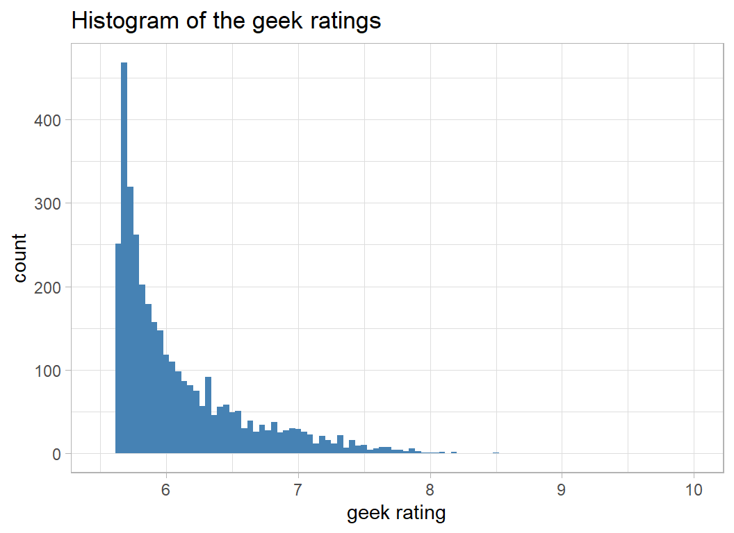
A log transformation would help to remove the skewness. The offset of 5.5, rather than 0 seems natural given the way that the ratings were created.
# --- transformed geek rating -------------------------
trainRawDF %>%
  ggplot( aes(x=log10(geek_rating - 5.5) ) ) +
  geom_histogram( bins=100, fill="steelblue") +
  labs(title="Histogram of the log transformed geek ratings")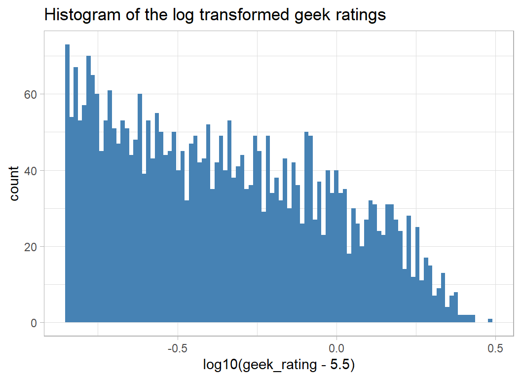
There is still a degree of skewness, but it does look as if the rating will be easier to model on this scale.
Votes and Owners
The method of deriving the rating suggests that there should be a relationship between geek_rating and num_votes and this is certainly the case.
Log transforming the number of votes makes this relationship clearer.
# --- log transformed rating and votes -----------------
trainRawDF %>%
  ggplot( aes(x=log10(num_votes), y=log10(geek_rating - 5.5)) ) +
  geom_point(colour="steelblue") +
  labs(title="Relationship between log transformed votes and rating")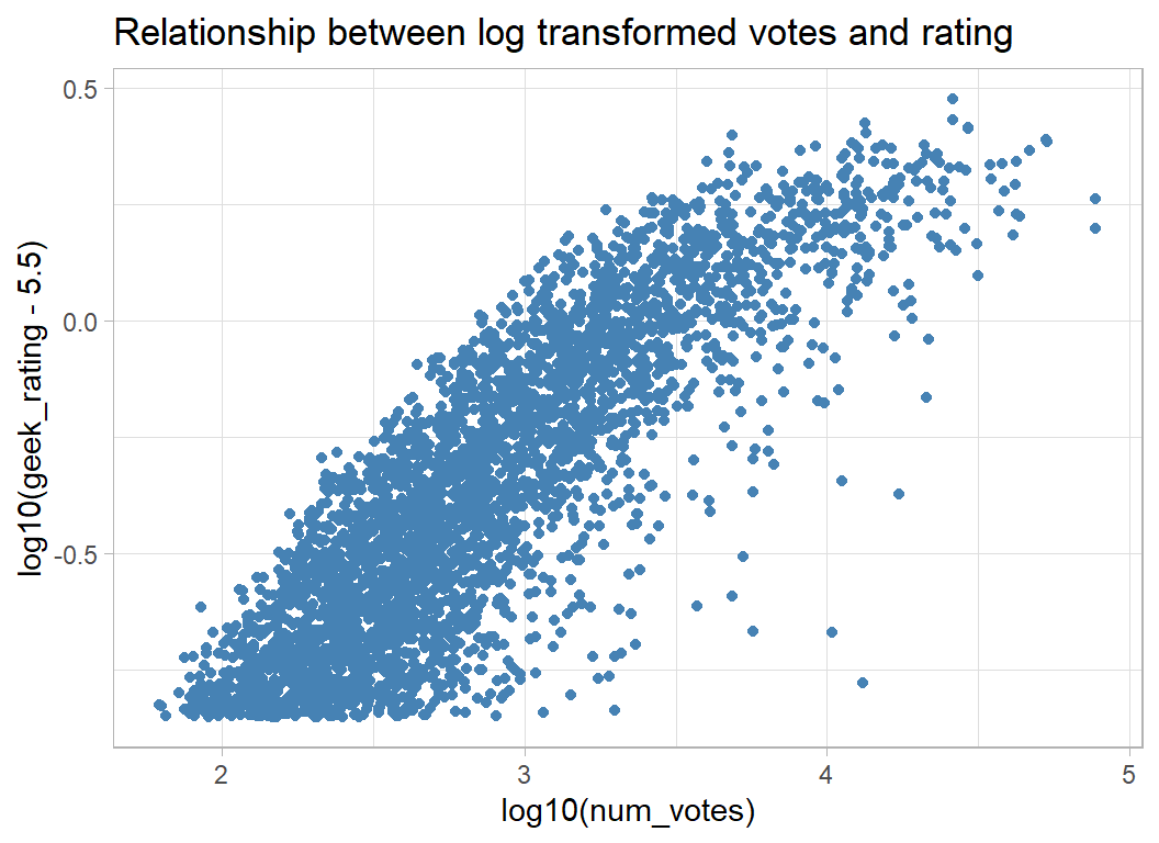
The evaluation of performance is made in terms of the RMSE of the prediction of geek_rating, which argues for working on the original scale, but my suspicion is that linear models will fit better on a log scale and it is a simple matter to convert the predictions back to the original scale.
As you might expect, the number of votes is closely related to, owned, the number of people who own the game.
# --- votes and number who own the game -----------------
trainRawDF %>%
  ggplot( aes(x=log10(owned), y=log10(num_votes)) ) +
  geom_point(colour="steelblue")  +
  labs( title="Relationship between votes and ownership")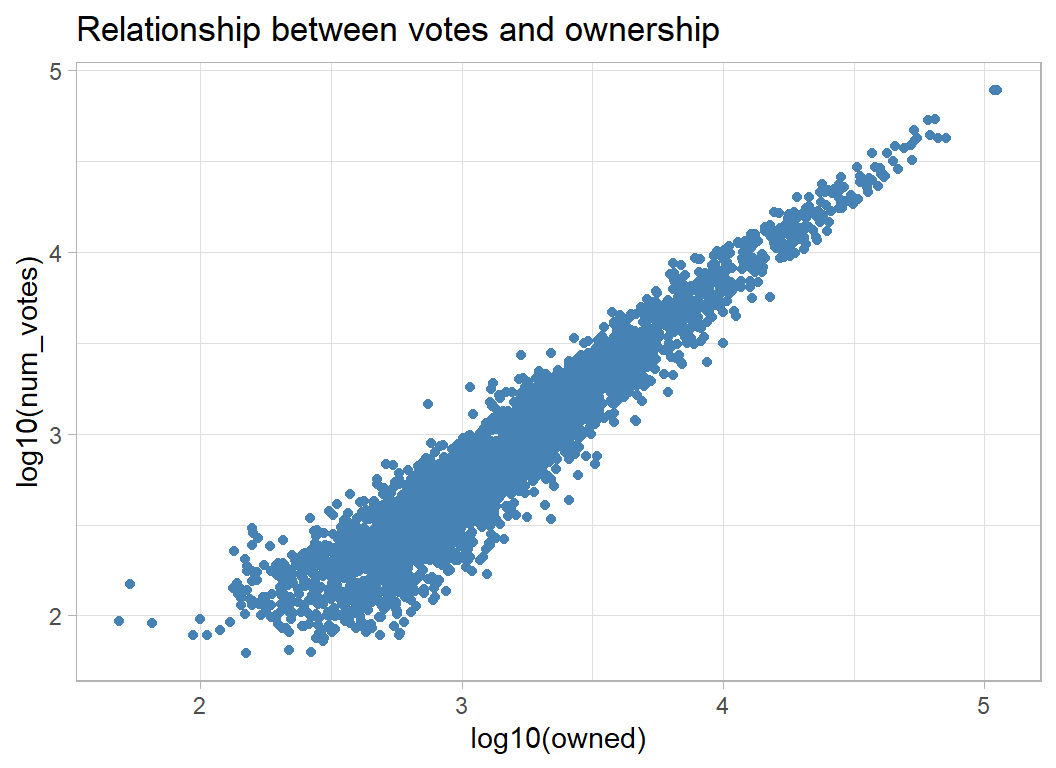
As a consequence, owned and num_votes are related to geek_rating in a similar way. People buy games that they are likely to enjoy, so widely owned games get higher ratings.
# --- ownership and geek rating -------------------------
trainRawDF %>%
  ggplot( aes(x=log10(owned), y=log10(geek_rating - 5.5)) ) +
  geom_point(colour="steelblue") +
  labs( title="Relationship between ownership and geek rating")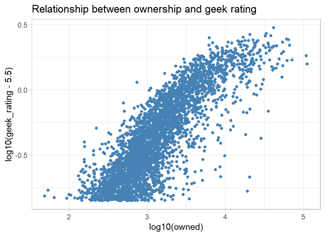
Other predictors
In later episodes, the contestants were given a data dictionary to explain the features, but for this episode we are left to guess. I take it that age refers to the minimum age that the game is aimed at.
# --- age and geek rating -------------------------
trainRawDF %>%
  ggplot( aes(x=age, y=log10(geek_rating - 5.5)) ) +
  geom_point(colour="steelblue") +
  labs( title="Relationship between age and geek rating")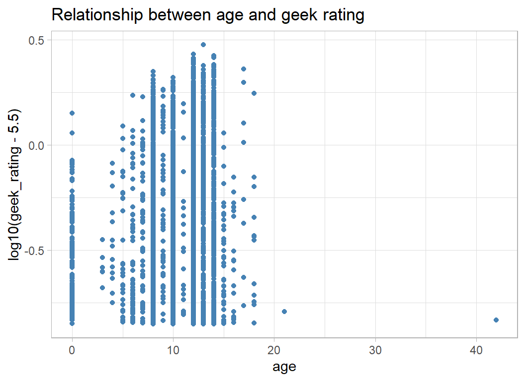
Lots of zeros, perhaps these are games without a minimum advised age. There is also a very odd 42.
Next the year of release
# --- year and geek rating -------------------------
trainRawDF %>%
  ggplot( aes(x=year, y=log10(geek_rating - 5.5)) ) +
  geom_point(colour="steelblue") +
  labs( title="Relationship between age and geek rating")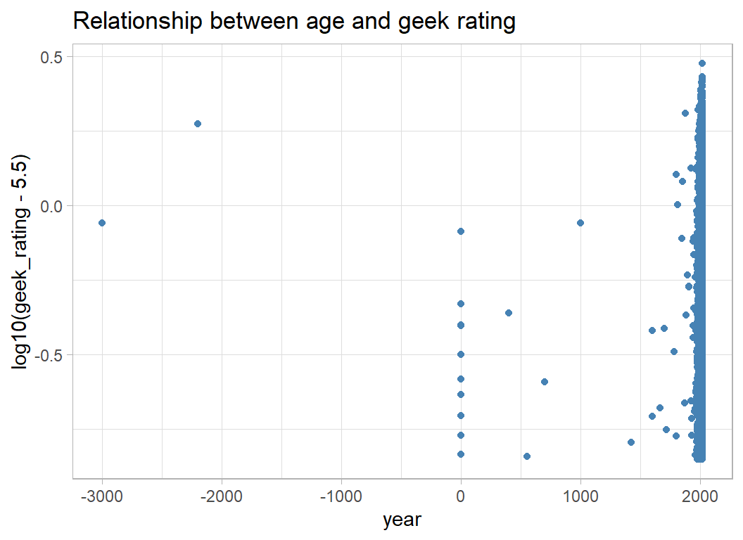
There is a weak pattern that is lost because of the bunching of recent games. Truncating the data at 1970 helps make the pattern clearer.
# --- truncated year and geek rating -------------------------
trainRawDF %>%
  mutate( year = pmax(1970, year)) %>%
  ggplot( aes(x=year, y=log10(geek_rating - 5.5)) ) +
  geom_point(colour="steelblue") +
  geom_smooth( colour="red") +
  labs( title="Relationship between truncated year and geek rating")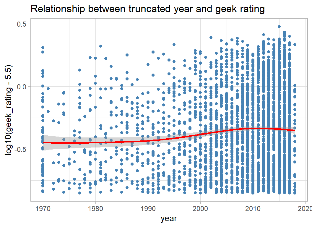
Next comes average time taken to play the game. Some games do take a long time, but 10,000 minutes is equivalent to a week of continuous play, which is hard to believe. Once again there are a few zeros.
# --- time to play and geek rating -------------------------
trainRawDF %>%
  ggplot( aes(x=log10(avg_time+1), y=log10(geek_rating - 5.5)) ) +
  geom_point(colour="steelblue") +
  geom_smooth( colour="red") +
  labs( title="Relationship between average time to play and geek rating")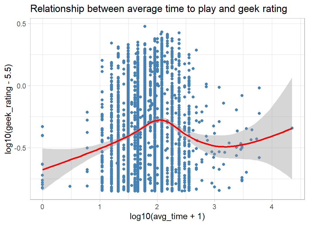
Number of players also has some extreme values
# --- players and geek rating -------------------------
trainRawDF %>%
  ggplot( aes(x=max_players, y=log10(geek_rating - 5.5)) ) +
  geom_point(colour="steelblue") +
  labs( title="Relationship between number of players and geek rating")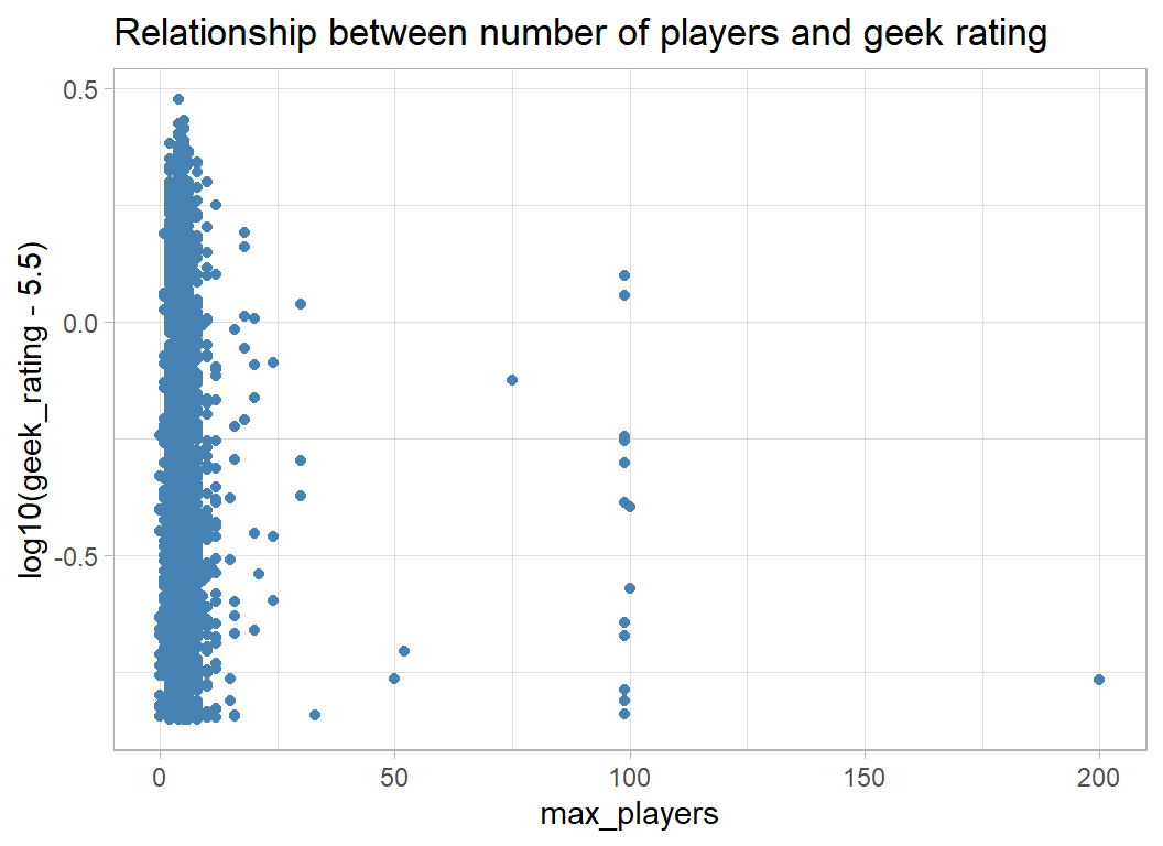
When the range is restricted to (1, 10), there is not much pattern, but perhaps games for fewer than 4 players are rated lower.
# --- players and geek rating -------------------------
trainRawDF %>%
  filter( max_players > 0 & max_players < 10 ) %>%
  mutate( max_players = factor(max_players)) %>%
  ggplot( aes(x=max_players, y=log10(geek_rating - 5.5)) ) +
  geom_boxplot(colour="steelblue") +
  labs( title="Relationship between number of players and geek rating")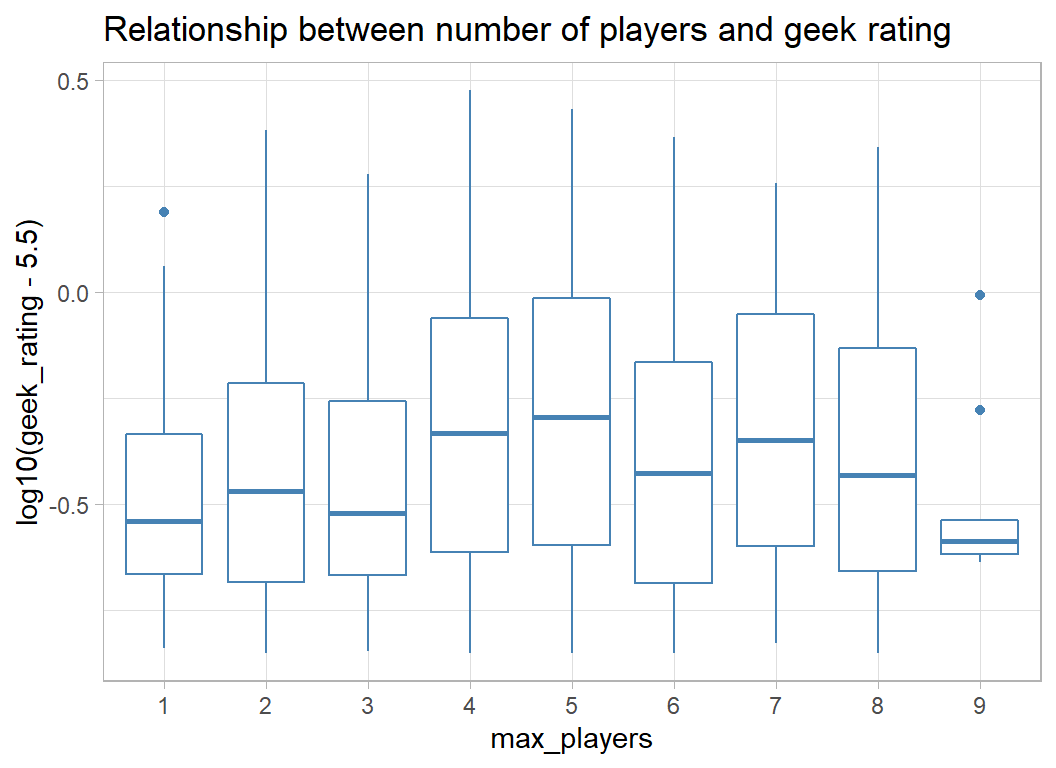
Unusual values
Let’s look at some of the unusual values, starting with the negative years
# --- unusual year game released --------------------------
trainRawDF %>%
  filter( year < 0 ) %>%
  select( game_id, names, year)
## # A tibble: 2 x 3
## game_id names year
## <dbl> <chr> <dbl>
## 1 2397 Backgammon -3000
## 2 188 Go -2200These are not unreasonable, backgammon has been around in some form for about 5000 years, taking us back to 3000BC and Go is also pretty old.
Here are the games with max_players equal to zero.
# --- zero number of players -----------------------------
trainRawDF %>%
  filter( max_players == 0 ) %>%
  select( game_id, names, min_players, max_players)
## # A tibble: 16 x 4
## game_id names min_players max_players
## <dbl> <chr> <dbl> <dbl>
## 1 60815 Black Powder 2 0
## 2 10904 New Rules for Classic Games 0 0
## 3 21804 Traditional Card Games 0 0
## 4 163097 Beyond the Rhine 2 0
## 5 174298 Napoleon's Last Gamble 2 0
## 6 5985 Miscellaneous Game Accessory 0 0
## 7 85204 Kings of War 2 0
## 8 23953 Outside the Scope of BGG 0 0
## 9 25738 The Big Taboo 4 0
## 10 37301 Decktet 0 0
## 11 2860 Piecepack 0 0
## 12 157323 MBT (second edition) 2 0
## 13 170669 Old School Tactical 2 0
## 14 197333 Deadzone (second edition) 2 0
## 15 18291 Unpublished Prototype 0 0
## 16 4292 The Sword and the Flame 0 0The list of games has a few non-specific titles including Traditional Card Games and Outside the Scope of BGG. Black Powder is a a classic battle reconstruction game with small model soldiers and max_players=0 seems to be either an error, or a way of saying that there is no maximum number of players.
A similar picture is seen when we look at the games that take no time to play
# --- zero time to play ---------------------------------
trainRawDF %>%
  filter( max_time == 0 ) %>%
  select( game_id, names, min_time, max_time)
## # A tibble: 44 x 4
## game_id names min_time max_time
## <dbl> <chr> <dbl> <dbl>
## 1 60815 Black Powder 0 0
## 2 10904 New Rules for Classic Games 0 0
## 3 21804 Traditional Card Games 0 0
## 4 280 Neue Spiele im alten Rom 0 0
## 5 206931 Noch mal! 20 0
## 6 222887 Twin It! 0 0
## 7 227758 Kokoro: Avenue of the Kodama 30 0
## 8 216658 Smash Up: What Were We Thinking? 45 0
## 9 224710 Zombicide: Green Horde 60 0
## 10 12071 Second Season Pro Football Game 120 0
## # ... with 34 more rowsSome of the max_players data is doubtful. Amazon tells me that Linkee is a card game for 2-30 players.
# --- very high max_players -----------------------------
trainRawDF %>%
  filter( max_players > 90 ) %>%
  select( game_id, names, min_players, max_players)
## # A tibble: 14 x 4
## game_id names min_players max_players
## <dbl> <chr> <dbl> <dbl>
## 1 233867 Welcome To... 1 100
## 2 30618 Eat Poop You Cat 3 99
## 3 155689 Dungeons & Dragons: Attack Wing 2 99
## 4 4985 Warmaster 2 99
## 5 163377 Rolling Japan 1 99
## 6 179217 Wonky 2 99
## 7 147194 Linkee 2 200
## 8 51 Ricochet Robots 1 99
## 9 131183 Wings of Glory: WW2 Rules and Accessories Pa~ 2 99
## 10 1519 Kult 2 99
## 11 119866 Wings of Glory: WW1 Rules and Accessories Pa~ 2 99
## 12 5614 Achtung: Spitfire! 1 99
## 13 32901 Prawo Dzungli 2 100
## 14 99875 Martian Dice 2 99Here are some extremely long game times.
# --- very long time to play ---------------------------------
trainRawDF %>%
  filter( avg_time > 1000 ) %>%
  select( game_id, names, avg_time, min_time, max_time)
## # A tibble: 32 x 5
## game_id names avg_time min_time max_time
## <dbl> <chr> <dbl> <dbl> <dbl>
## 1 5622 Pacific War 6000 60 6000
## 2 163097 Beyond the Rhine 3000 3000 3000
## 3 1563 Rise and Decline of the Third Reich 1440 1440 1440
## 4 27817 Marne 1918: Friedensturm 1200 0 1200
## 5 29285 Case Blue 22500 0 22500
## 6 94373 Dien Bien Phu: The Final Gamble 1440 0 1440
## 7 1499 World in Flames 6000 120 6000
## 8 193238 Tunisia II 3000 120 3000
## 9 70532 Tonkin: The Indochina war 1950-54 (second~ 1800 0 1800
## 10 7614 A World at War 2880 1440 2880
## # ... with 22 more rowsCase Blue is a political strategy game that BGG says can last between 1440 and 22500 minutes. This takes some believing, but even if it were true the minimum time is not 0 minutes and the average must be less than 22500.
Text analysis
The fields mechanic and category1 to category12 contain structured text that describes the way that the game is played and the type of game. In the case of mechanic the information is contained in a single column with a comma separator.
# --- game mechanics -------------------------------------
trainRawDF %>%
  select( mechanic)
## # A tibble: 3,499 x 1
## mechanic
## <chr>
## 1 Hand Management
## 2 Point to Point Movement, Route/Network Building
## 3 Betting/Wagering, Dice Rolling, Roll / Spin and Move
## 4 Secret Unit Deployment, Simultaneous Action Selection
## 5 Action Point Allowance System, Dice Rolling, Modular Board, Partnerships, Va~
## 6 Hand Management, Take That
## 7 Action Point Allowance System, Memory
## 8 Dice Rolling, Hex-and-Counter
## 9 Co-operative Play, Dice Rolling, Simulation
## 10 Dice Rolling, Hand Management
## # ... with 3,489 more rowsIn contrast, the categories are spread over 12 columns so no separator is needed. Here are the first few entries.
# --- game categorisation --------------------------------
trainRawDF %>%
  select( category1, category2, category3)
## # A tibble: 3,499 x 3
## category1 category2 category3
## <chr> <chr> <chr>
## 1 Card Game Collectible Components Horror
## 2 Animals Exploration Transportation
## 3 Abstract Strategy Dice <NA>
## 4 Bluffing Card Game City Building
## 5 Adventure Exploration Fantasy
## 6 Card Game Modern Warfare Nautical
## 7 Animals Children's Game Maze
## 8 Modern Warfare Nautical Wargame
## 9 Science Fiction <NA> <NA>
## 10 City Building Medieval <NA>
## # ... with 3,489 more rowsIt is difficult to incorporate text features into a statistical model, so I replace the most informative entries by indicator variables.
The code below identifies the most common entries for mechanic. A few rows have more than 6 game mechanics, which I ignore.
# --- common words describing the game mechanic ------------
trainRawDF %>%
  select(game_id, mechanic) %>%
  # --- extract the first six entries ---
  separate(mechanic,
           into = c("m1", "m2", "m3", "m4", "m5", "m6"),
           sep  = "," ) %>%
  # --- stack m1 to m6 ---
  pivot_longer(m1:m6,
               values_to = "items",
               names_to  = "source" ) %>%
  # --- drop any missing values ---
  filter( !is.na(items) ) %>%
  # --- trim unwanted white space ---
  mutate( items = str_trim(items)) %>%
  # --- remove the 'none' category ---
  filter( items != "none" ) %>%
  # --- arrange by frequency ---
  count( items, sort=TRUE) %>%
  # --- remove rare mechanics ---
  filter( n >= 25 ) %>%
  # --- extract to a character vector ---
  print() %>%
  pull( items ) -> mecWords
## # A tibble: 45 x 2
## items n
## <chr> <int>
## 1 Dice Rolling 990
## 2 Hand Management 961
## 3 Variable Player Powers 580
## 4 Set Collection 506
## 5 Area Control / Area Influence 446
## 6 Card Drafting 415
## 7 Modular Board 398
## 8 Tile Placement 377
## 9 Hex-and-Counter 317
## 10 Action Point Allowance System 287
## # ... with 35 more rowsPredictably, dice rolling is the most common mechanic featuring in 990 of the 3499 games.
For each of the 45 mechanics that occur at least 25 times, a t-test of (transformed) geek_rating is used to compare the mean rating of games with that mechanic (mWith) to the mean of games without it (mWithout).
# --- Tibble for the results --------------------------
tibble( mechanic = mecWords,
        p_value  = double(45),
        mWithout = double(45),
        mWith    = double(45)) -> mecDF
# --- 45 t-tests --------------------------------------
for( i in 1:45 ) {
  # --- create an indicator ---------------------------
  trainRawDF %>%
    mutate( y = log10(geek_rating-5.5) ) %>%
    mutate( class = as.numeric(str_detect(mechanic, mecWords[i]))) -> tDF

  # --- t-test and mean geek ratings ------------------
  mecDF$p_value[i]  <- t.test(tDF$y ~ tDF$class )$p.value
  mecDF$mWithout[i] <- mean(tDF$y[tDF$class==0])
  mecDF$mWith[i]    <- mean(tDF$y[tDF$class==1])
}
# --- sort and display --------------------------------
mecDF %>%
  arrange(p_value) %>%
  print() -> mecDF
## # A tibble: 45 x 4
## mechanic p_value mWithout mWith
## <chr> <dbl> <dbl> <dbl>
## 1 Hex-and-Counter 5.14e-33 -0.341 -0.536
## 2 Variable Player Powers 3.69e-21 -0.386 -0.241
## 3 Card Drafting 2.04e-16 -0.377 -0.225
## 4 Area Control / Area Influence 1.35e-15 -0.377 -0.238
## 5 Hand Management 1.10e-14 -0.386 -0.287
## 6 Chit-Pull System 3.38e-12 -0.355 -0.582
## 7 Worker Placement 1.39e-11 -0.370 -0.207
## 8 Deck / Pool Building 1.16e- 9 -0.368 -0.221
## 9 Grid Movement 3.16e- 8 -0.368 -0.231
## 10 Action Point Allowance System 1.29e- 7 -0.368 -0.256
## # ... with 35 more rowsSo Hex-and-Counter games have an average transformed rating of -0.536 (geometric average geek rating 10^-0.536 + 5.5 = 5.79) as opposed to -0.341 (rating=5.96) for games that do not use Hex-and-Counter, a very significant difference.
I wanted to do much the same thing for categories and designers, so I wrote a function that does all this in one go; it is called select_indicators(). In order not to interrupt the flow, I’ve given the code for the function as an appendix at the end of this post.
Let’s reassure ourselves that the function gives the same results for mechanic
# --- test the function on mechanic ---------------
trainRawDF %>%
  mutate( mechanic = str_replace_all(mechanic, "none", "")) %>%
  mutate( log_rating = log10(geek_rating-5.5) ) %>%
  select_indicators(mechanic, log_rating) %>%
  print() -> mecDF
## # A tibble: 45 x 5
## term count p_value mWithout mWith
## <chr> <int> <dbl> <dbl> <dbl>
## 1 Hex-and-Counter 317 5.14e-33 -0.341 -0.536
## 2 Variable Player Powers 646 3.69e-21 -0.386 -0.241
## 3 Card Drafting 415 2.04e-16 -0.377 -0.225
## 4 Area Control / Area Influence 446 1.35e-15 -0.377 -0.238
## 5 Hand Management 963 1.10e-14 -0.386 -0.287
## 6 Chit-Pull System 57 3.38e-12 -0.355 -0.582
## 7 Worker Placement 244 1.39e-11 -0.370 -0.207
## 8 Deck / Pool Building 209 1.16e- 9 -0.368 -0.221
## 9 Grid Movement 224 3.16e- 8 -0.368 -0.231
## 10 Action Point Allowance System 287 1.29e- 7 -0.368 -0.256
## # ... with 35 more rowsThe results tally with what we had before, so now we can do the same for categories by first uniting all the categories into a single column.
# --- categorisations -----------------------------
trainRawDF %>%
  unite( "category", category1:category12, sep=" , ",
         remove=TRUE, na.rm=TRUE) %>%
  mutate( log_rating = log10(geek_rating-5.5) ) %>%
  select_indicators(category, log_rating) %>%
  print() -> catDF
## # A tibble: 64 x 5
## term count p_value mWithout mWith
## <chr> <int> <dbl> <dbl> <dbl>
## 1 Economic 395 5.88e-15 -0.376 -0.226
## 2 Wargame 635 1.44e-13 -0.341 -0.442
## 3 World War I 265 1.23e-10 -0.350 -0.466
## 4 City Building 171 1.74e- 9 -0.367 -0.201
## 5 Fighting 380 2.33e- 9 -0.372 -0.255
## 6 World War II 221 1.04e- 8 -0.352 -0.462
## 7 Children's Game 105 7.08e- 7 -0.355 -0.494
## 8 Civilization 115 1.99e- 6 -0.364 -0.197
## 9 Industry / Manufacturing 90 2.05e- 6 -0.364 -0.181
## 10 Renaissance 89 3.71e- 6 -0.364 -0.184
## # ... with 54 more rowsThe geeks are surprisingly pacifist. City Building is rated higher than Wargames.
Finally, I will look at the designers. There are a few oddities that have to be handled before we use select_indicators(). A name such as “Fred Blogs, Jr” already contains a comma, which we are using as the separator, so those commas have to go. Next, there are a few names that include brackets such as “Fred Blogs (I)”. Brackets cause havoc, because they are special characters in regex, so they too have to go.
# --- the effect of designer -----------------------------
trainRawDF %>%
  mutate( designer = str_replace(designer, ", Jr", "Jr")) %>%
  mutate( designer = str_replace_all(designer, "\\(", "")) %>%
  mutate( designer = str_replace_all(designer, "\\)", "")) %>%
  mutate( log_rating = log10(geek_rating-5.5) ) %>%
  select_indicators(designer, log_rating) %>%
  print() -> desDF
## # A tibble: 11 x 5
## term count p_value mWithout mWith
## <chr> <int> <dbl> <dbl> <dbl>
## 1 Dean Essig 33 0.0000000174 -0.357 -0.582
## 2 Richard H. Berg 26 0.000951 -0.358 -0.513
## 3 Mike Elliott 27 0.00132 -0.360 -0.164
## 4 Bruno Cathala 31 0.00148 -0.361 -0.155
## 5 Martin Wallace 41 0.00339 -0.361 -0.204
## 6 Wolfgang Kramer 38 0.00944 -0.360 -0.219
## 7 Alan R. Moon 32 0.105 -0.360 -0.278
## 8 Friedemann Friese 27 0.173 -0.360 -0.273
## 9 Reiner Knizia 85 0.461 -0.360 -0.334
## 10 Uncredited 52 0.630 -0.359 -0.380
## 11 Klaus Teuber 26 0.944 -0.359 -0.363Rather depressing for those designers who have below average ratings.
Is it worth using the designers given the low counts and the small difference that they make to the mean?
We have a training set of about 3500 games and the RMSE is, ballpark, 0.2. This makes the MSE=0.04 and the sum of squares of the prediction errors 3500x0.04=140. Suppose that including a designer of 30 games makes the predictions perfect for those 30 games. The sum of squares would be expected to reduce to 3470x0.04=138.8. So the new MSE would be 0.0397 and the RMSE would reduce from 0.200 to 0.199. Who cares?
Well, it might be important to include a designer if you were thinking of investing in their next game, but for accuracy of prediction such infrequent indicator variables are a waste of time, unless of course, you are trying to win a prediction competition. I’ll not be using the designer.
Data Cleaning
The numbers of improbable zeros is quite small and hardly justifies an elaborate imputation. However, I am a little concerned that the zeros might influence the predictions, so I replace them by the median. I also replace the extreme years and extreme ages.
I wrote a function called make_indictors() that makes indicator variables out of a text field and this too is given in the appendix.
Of course, we need to treat the training and test data identically. Here is my data cleaning code applied to both datasets.
# --- DATA CLEANING ------------------------------------
#

# --- values for imputation ----------------------------
mnp <- median( trainRawDF$min_players)
mxp <- median( trainRawDF$max_players)
avt <- median( trainRawDF$avg_time)
mnt <- median( trainRawDF$min_time)
mxt <- median( trainRawDF$max_time)
mda <- median( trainRawDF$age)

# --- indicators for top 10 mechanics ------------------
imDF <- make_indicators(trainRawDF$mechanic,
                        mecDF$term[1:10], prefix="M")
# --- indicators for top 10 categories -----------------
icDF <- make_indicators(
             trainRawDF %>%
               unite( "cat", category1:category12,
                      sep=" ", remove=TRUE, na.rm=TRUE) %>%
               pull(cat) ,
             catDF$term[1:10], prefix="C")

# --- clean training data -------------------------------
trainRawDF %>%
  # --- impute zero values --------------------------------------
  mutate( min_players = ifelse(min_players==0, mnp, min_players),
          max_players = ifelse(max_players==0, mxp, max_players),
          avg_time    = ifelse(avg_time==0   , avt, avg_time),
          min_time    = ifelse(min_time==0   , mnt, min_time),
          max_time    = ifelse(max_time==0   , mxt, max_time),
          age         = ifelse(age==0        , mda, age)        ) %>%
  # --- truncate extreme values --------------------------------
  mutate( year        = pmax( 1970, year),
          max_players = pmin( 25, max_players),
          max_time    = pmin( 1000, max_time),
          avg_time    = pmin( (min_time+max_time)/2, avg_time),
          age         = pmin(age, 18) ) %>%
  # --- add indicators ---------------------
  bind_cols( imDF) %>%
  bind_cols( icDF) %>%
  # --- drop unwanted text columns ---------
  select( -mechanic, -starts_with("cat"), -designer ) %>%
  # --- save clean data --------------------
  saveRDS( file.path(home, "data/rData/clean_train.rds"))

# --- REPEAT FOR THE TEST DATA -----------------------------------
imDF <- make_indicators(testRawDF$mechanic,
                        mecDF$term[1:10], prefix="M")
icDF <- make_indicators(
             testRawDF %>%
               unite( "cat", category1:category12,
                      sep=" ", remove=TRUE, na.rm=TRUE) %>%
               pull(cat) ,
             catDF$term[1:10], prefix="C")

testRawDF %>%
  # --- impute zero values --------------------------------------
  mutate( min_players = ifelse(min_players==0, mnp, min_players),
          max_players = ifelse(max_players==0, mxp, max_players),
          avg_time    = ifelse(avg_time==0   , avt, avg_time),
          min_time    = ifelse(min_time==0   , mnt, min_time),
          max_time    = ifelse(max_time==0   , mxt, max_time),
          age         = ifelse(age==0        , mda, age)        ) %>%
  # --- truncate extreme values --------------------------------
  mutate( year        = pmax( 1970, year),
          max_players = pmin( 25, max_players),
          max_time    = pmin( 1000, max_time),
          avg_time    = pmin( (min_time+max_time)/2, avg_time),
          age         = pmin(age, 18) ) %>%
  # --- add text indicators ------------------------------------
  bind_cols( imDF) %>%
  bind_cols( icDF) %>%
  # --- drop unwanted text columns ---------
  select( -mechanic, -starts_with("cat"), -designer ) %>%
  # --- save clean data --------------------
  saveRDS( file.path(home, "data/rData/clean_test.rds"))
Data Splitting
I start by reading the cleaned training data and splitting it into a training and a validation set. The validation set is for assessing whether we are over-fitting. Cross-validation is more accurate because it averages over multiple validation datasets, but it is also slower. I could, perhaps, switch to cross-validation if I have to make fine distinctions between possible models.
In the code below, I split the cleaned version of trainRawDF (n=3499) into estimateDF (n=2499) and validateDF (n=1000). There are several packages that include functions for splitting into estimation and validation data, but the task is so simple that there is no real need to use them.
Most of the predictors are quite skew, so they are easier to use if they are log transformed. I do this en masse.
# --- read clean training data ------------------------------
readRDS( file.path(home, "data/rData/clean_train.rds")) %>%
  mutate( geek_rating = log10(geek_rating - 5.5),
          owned       = log10(owned),
          num_votes   = log10(num_votes),
          min_players = log10(min_players),
          max_players = log10(max_players),
          min_time    = log10(min_time),
          max_time    = log10(max_time),
          avg_time    = log10(avg_time)) -> trainDF

# --- randomly select 1000 rows for validation --------------
set.seed(8922)
split <- sample(1:nrow(trainDF), size=1000, replace=FALSE)

# --- split the data ---------------------------------i--
validateDF <- trainDF[  split, ]
estimateDF <- trainDF[ -split, ]
Information leakage
I used the full training set to select the most important words from the text variables and to calculated the medians for imputation. Since the validation set is a subset of the training set, the validation data have influenced this preprocessing. In other words, information will have leaked from validation set into the model fitting. As a result, performance of the predictions in the validation data will be slightly optimistic.
The correct procedure would be to rerun the data cleaning on the estimation set, but would it make a difference? Possibly one of the selected words would change, or the medians used for imputation might be very slightly different, but I find it hard to believe that these effects would important. It is a matter of judgement, but I am more concerned about the dubious data and the fact that I used median for imputation rather than chained equations.
Linear models
Let’s give ourselves a baseline by calculating the standard deviation of geek_rating, this is equivalent to the RMSE of a model that predicted that every game would get the same average rating. The standard deviation of the ratings in the estimation set is 0.481. This is our starting point. The aim, as represented by the leaderboard on the kaggle site, is to get the RMSE below 0.2. The winning model scored 0.161.
A simple linear regression model that includes every available predictor ought to be a marked improvement of the average prediction. I’ll use the broom package to extract information about the fit.
library(broom)

# --- model with all predictors ----------------------------
estimateDF %>%
  select( -game_id, -names) %>%
  { lm( geek_rating ~ ., data=.) } -> mod

# --- goodness of fit measures -----------------------------
glance(mod)
## # A tibble: 1 x 12
## r.squared adj.r.squared sigma statistic p.value df logLik AIC BIC
## <dbl> <dbl> <dbl> <dbl> <dbl> <dbl> <dbl> <dbl> <dbl>
## 1 0.813 0.810 0.143 369. 0 29 1329. -2595. -2415.
## # ... with 3 more variables: deviance <dbl>, df.residual <int>, nobs <int>R-squared tells us that the model explains about 80% of the variance, which is very promising. However, sigma (an adjusted RMSE) is on the transformed scale. So, we need to back-transform the predictions in order to calculate the competition RMSE.
We will need to calculate the in-sample and out-of-sample RMSE for each of our models, so it will save code if we write a function that does the calculations.
# -- Function to calculate the RMSE -------------------------
# arguments
#    model  ... fitted model to be summarised
# returns
#    prints the in-sample and out-of-sample rmse on the original scale
#
metrics <- function(model) {

  # --- in-sample RMSE on the original scale ------------------
  estimateDF %>%
    mutate( .fitted = predict(model),
            yhat    = 5.5 + 10^.fitted,
            y       = 5.5 + 10^geek_rating) %>%
    summarise( RMSE = sqrt(mean( (y - yhat)^2)) ) %>%
    pull(RMSE) -> inRMSE

# --- validation RMSE ---------------------------------------
  validateDF %>%
    mutate( .fitted = predict(mod, newdata=.),
            yhat    = 5.5 + 10^.fitted,
            y       = 5.5 + 10^geek_rating) %>%
    summarise( RMSE = sqrt(mean( (y - yhat)^2)) ) %>%
    pull(RMSE) -> outRMSE

  return( cat(sprintf("Estimation RMSE:  %8.3f\nValidation RMSE:  %8.3f\n",
                 inRMSE, outRMSE)))
}
metrics(mod)
## Estimation RMSE: 0.264
## Validation RMSE: 0.278Since we have not excessively tuned this model, the in-sample (estimation) RMSE and the out-of-sample (validation) RMSE are similar. The reduction in RMSE from 0.481 to 0.278 corresponds to about 70% in the variance.
The table of coefficients shows which predictors are most important
# --- regression coefficients --------------------------
tidy(mod) %>%
  print(n=30)
## # A tibble: 30 x 5
## term estimate std.error statistic p.value
## <chr> <dbl> <dbl> <dbl> <dbl>
## 1 (Intercept) -10.9 0.626 -17.3 1.19e- 63
## 2 min_players -0.0510 0.0216 -2.36 1.82e- 2
## 3 max_players -0.102 0.0155 -6.58 5.86e- 11
## 4 avg_time 0.00331 0.0880 0.0376 9.70e- 1
## 5 min_time -0.0359 0.0358 -1.00 3.16e- 1
## 6 max_time 0.162 0.0595 2.73 6.43e- 3
## 7 year 0.00437 0.000312 14.0 4.46e- 43
## 8 num_votes 0.610 0.0224 27.3 3.23e-143
## 9 age 0.00553 0.00157 3.53 4.23e- 4
## 10 owned -0.0838 0.0243 -3.45 5.72e- 4
## 11 M1 0.00901 0.0147 0.611 5.41e- 1
## 12 M2 0.0163 0.00837 1.94 5.23e- 2
## 13 M3 0.00269 0.00935 0.287 7.74e- 1
## 14 M4 -0.00217 0.00899 -0.242 8.09e- 1
## 15 M5 -0.0146 0.00684 -2.14 3.28e- 2
## 16 M6 -0.0289 0.0242 -1.19 2.33e- 1
## 17 M7 0.0255 0.0125 2.03 4.22e- 2
## 18 M8 0.0717 0.0131 5.49 4.51e- 8
## 19 M9 0.0282 0.0124 2.27 2.31e- 2
## 20 M10 0.0241 0.0110 2.20 2.80e- 2
## 21 C1 0.0212 0.0107 1.99 4.68e- 2
## 22 C2 0.0401 0.0119 3.39 7.22e- 4
## 23 C3 -0.00650 0.0248 -0.262 7.94e- 1
## 24 C4 -0.00383 0.0144 -0.265 7.91e- 1
## 25 C5 -0.00383 0.0101 -0.379 7.05e- 1
## 26 C6 0.0144 0.0266 0.540 5.89e- 1
## 27 C7 0.0149 0.0179 0.832 4.06e- 1
## 28 C8 -0.00203 0.0165 -0.123 9.02e- 1
## 29 C9 0.0142 0.0197 0.722 4.71e- 1
## 30 C10 0.0141 0.0187 0.754 4.51e- 1As I anticipated, it is the number of votes that is most predictive. The text indicators don’t add much. The best are M8 (Deck/Pool Building) and C2 (Wargame).
A residual plot shows that there is pattern that has not been captured, especially at the extremes of the range of geek-rating.
# --- residual plot ------------------------------------
augment(mod) %>%
  ggplot( aes(x=.fitted, y=.resid)) +
  geom_point(colour="steelblue") +
  geom_hline(yintercept=0) +
  geom_smooth(colour="red") +
  labs( x="Predicted values", y="Residuals",
        title="Residual plot on the transformed rating scale")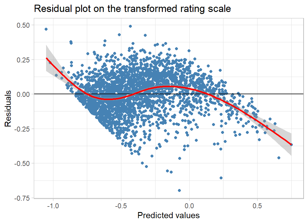
Plotting against num_votes (which is on a log scale) suggests that the under-prediction might be correctd by allowing for its non-linearity.
# --- residuals and votes --------------------------------
augment(mod) %>%
  ggplot(aes(x=num_votes, y = .resid)) +
  geom_point(colour="steelblue") +
  geom_smooth(colour="red") +
  geom_hline(yintercept=0)  +
  labs( x="log10(number of votes)", y="Residuals",
        title="Residuals against log10 number of votes")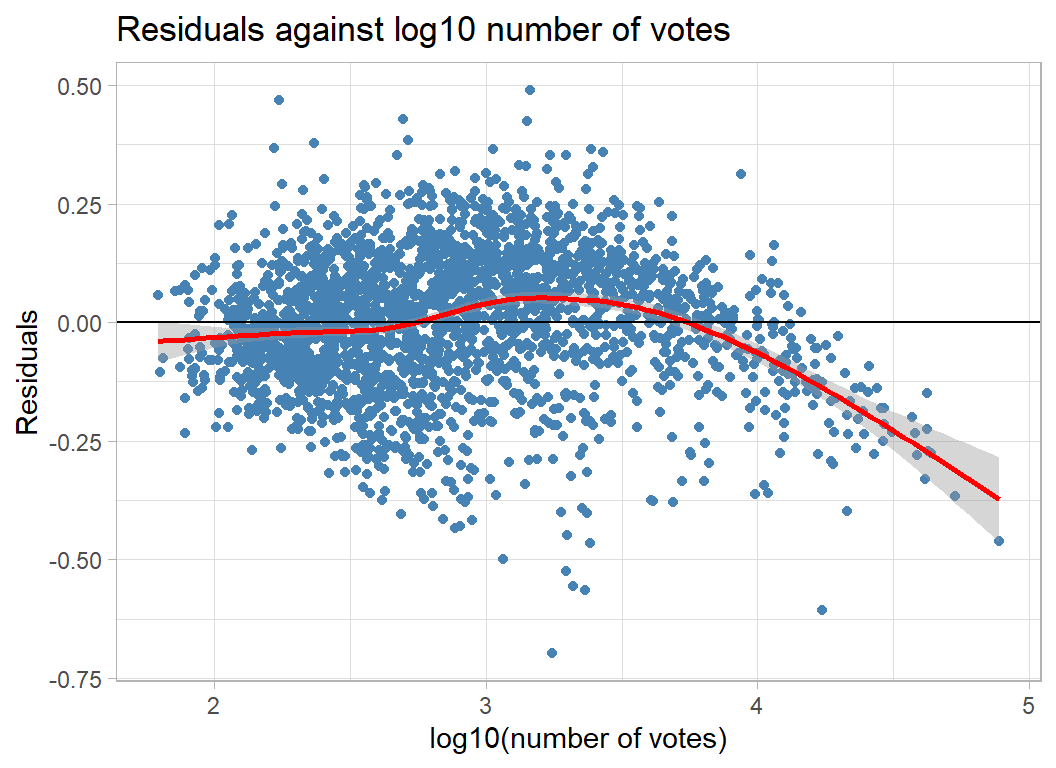
There is also non-linearity in the pattern of residual over years.
# --- residuals and year of release ----------------------
augment(mod) %>%
ggplot(aes(x=year, y = .resid)) +
geom_point(colour="steelblue") +
geom_smooth(colour="red") +
geom_hline(yintercept=0) +
labs( x="year", y="Residuals",
title="Residuals against year of release")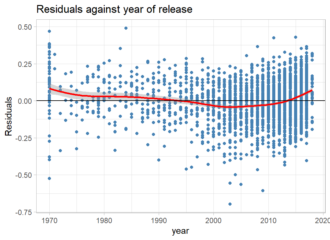 It may be important to allow for non-linearity in these and other continuous variables.
Generalised Additive Models
A Generalised Additive Model (GAM) is a linear model in which the relationships between the response and the continuous predictors are represented by smooth functions, usually splines. The main problem when fitting a GAM is to decide how smooth to make the splines.
There are two packages in R that will fit GAMs, gam and mgcv. The big advantage of mgcv is that it incorporates methods for estimating the degree of smoothness. The package’s default is to use a cross-validation approach.
mgcv is a complex package, to get some idea of the complexity you might look at the package author’s own slides at https://www.maths.ed.ac.uk/~swood34/mgcv/SmoothModels.pdf. They include a very nice explanation of splines as sums of basis functions with a smoothness penalty.
As with all methods of analysis, if you do not understand it, don’t use it; but, this advice does not mean that you have to understand every nuance, that way you would be paralysed and you would never advance. You do need to understand the general approach and the specifics of the options that you choose.
The next model uses splines for the continuous variables and includes the top 10 indicators of mechanics and the top 10 indicators of category. I’ve not placed a spline on min_players because the range is so small. It might have been better to treat min_players as a factor.
library(mgcv)

# --- fit a GAM -----------------------------------------------------
estimateDF %>%
  { gam( geek_rating ~ min_players + s(max_players) +
           s(min_time) + s(max_time) + s(avg_time) +
           s(year) + s(num_votes) + s(age) + s(owned) +
           M1 + M2 + M3 + M4 + M5 + M6 + M7 + M8 + M9 + M10 +
           C1 + C2 + C3 + C4 + C5 + C6 + C7 + C8 + C9 + C10 , data=.) } -> mod

metrics(mod)
## Estimation RMSE: 0.164
## Validation RMSE: 0.174So we are already at 0.174, which is competitive with the leaderboard. To get into the top 5 we would need a RMSE (in the test data) below 0.17.
Here are the p-values for each term
# --- analysis of variance -----------------------------------------
anova(mod)
##
## Family: gaussian
## Link function: identity
##
## Formula:
## geek_rating ~ min_players + s(max_players) + s(min_time) + s(max_time) +
## s(avg_time) + s(year) + s(num_votes) + s(age) + s(owned) +
## M1 + M2 + M3 + M4 + M5 + M6 + M7 + M8 + M9 + M10 + C1 + C2 +
## C3 + C4 + C5 + C6 + C7 + C8 + C9 + C10
##
## Parametric Terms:
## df F p-value
## min_players 1 1.561 0.21159
## M1 1 9.562 0.00201
## M2 1 0.893 0.34478
## M3 1 0.591 0.44199
## M4 1 2.357 0.12485
## M5 1 1.223 0.26890
## M6 1 0.009 0.92427
## M7 1 0.096 0.75713
## M8 1 19.130 1.27e-05
## M9 1 3.670 0.05552
## M10 1 2.986 0.08411
## C1 1 9.652 0.00191
## C2 1 19.732 9.31e-06
## C3 1 0.006 0.93685
## C4 1 0.468 0.49383
## C5 1 1.188 0.27589
## C6 1 0.090 0.76375
## C7 1 0.028 0.86645
## C8 1 0.008 0.92776
## C9 1 0.037 0.84678
## C10 1 1.018 0.31318
##
## Approximate significance of smooth terms:
## edf Ref.df F p-value
## s(max_players) 8.355 8.776 22.984 <2e-16
## s(min_time) 1.000 1.000 0.915 0.3389
## s(max_time) 1.334 1.612 0.071 0.8775
## s(avg_time) 1.000 1.000 5.126 0.0237
## s(year) 8.333 8.846 70.026 <2e-16
## s(num_votes) 1.963 2.521 513.299 <2e-16
## s(age) 4.960 5.971 3.644 0.0013
## s(owned) 4.697 5.831 32.135 <2e-16Clearly, num_votes is the key, along with owned, year, and max_players. There are also contributions from avg_time, age, M1, M8, M9, M10, C1 and C2.
Here is a simpler model without the non-significant features. I am more confident that these relationships are real.
# --- fit a simpler GAM ----------------------------------------------
estimateDF %>%
  { gam( geek_rating ~ s(max_players) + s(avg_time) +
           s(year) + s(num_votes) + s(age) + s(owned) +
           M1 + M8 + M9 + M10 +
           C1 + C2    , data=.) } -> mod

# --- RMSE -----------------------------------------------------------
metrics(mod)
## Estimation RMSE: 0.165
## Validation RMSE: 0.175# --- Analysis of Variance -------------------------------------------
anova(mod)##
## Family: gaussian
## Link function: identity
##
## Formula:
## geek_rating ~ s(max_players) + s(avg_time) + s(year) + s(num_votes) +
## s(age) + s(owned) + M1 + M8 + M9 + M10 + C1 + C2
##
## Parametric Terms:
## df F p-value
## M1 1 11.259 0.000804
## M8 1 21.925 2.99e-06
## M9 1 5.606 0.017977
## M10 1 3.359 0.066962
## C1 1 10.000 0.001584
## C2 1 19.447 1.08e-05
##
## Approximate significance of smooth terms:
## edf Ref.df F p-value
## s(max_players) 8.630 8.918 23.176 < 2e-16
## s(avg_time) 2.799 3.615 74.128 < 2e-16
## s(year) 8.264 8.814 87.697 < 2e-16
## s(num_votes) 2.008 2.606 508.225 < 2e-16
## s(age) 5.002 5.995 4.598 0.000127
## s(owned) 5.584 6.789 27.299 < 2e-16The RMSE in the validation sample is very similar to that obtained for the full set of predictors. Remember that performance is being measured in a single validation sample, it would take a large scale cross-validation to choose between such similar models. My default is to prefer the simpler model.
The effective degrees of freedom (edf) for num_votes is 2.0 telling us that it is treated like a quadratic. The misrepresentation of the rating for very high num_votes seems to have been picked up by the closely related owned predictor. Presumably, we could obtain very similar predictions from a model in which the roles of owned and num_votes were reversed.
The mgcv package includes a function for producing model plots that enables the user to picture the shapes of the relationships. Unfortunately, the plots are created with base R graphics.
plot(mod, scale=0, residuals=TRUE)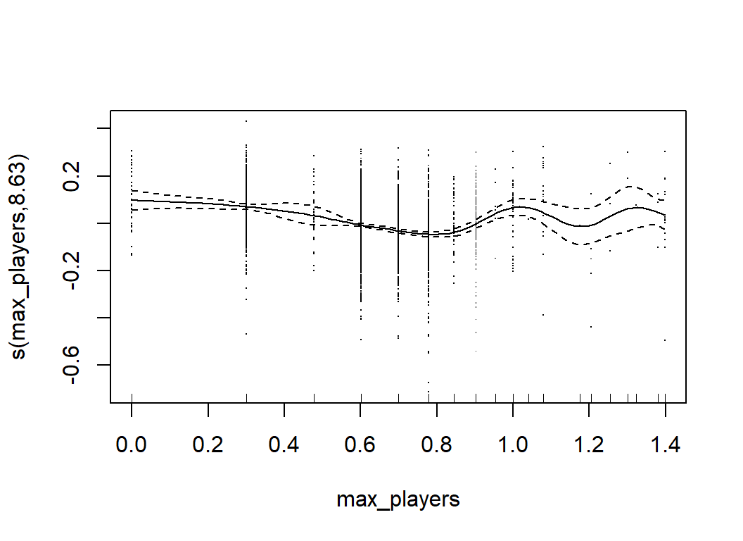
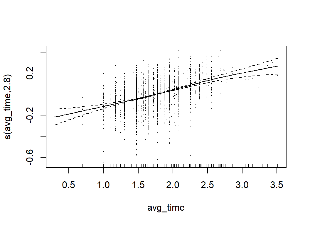
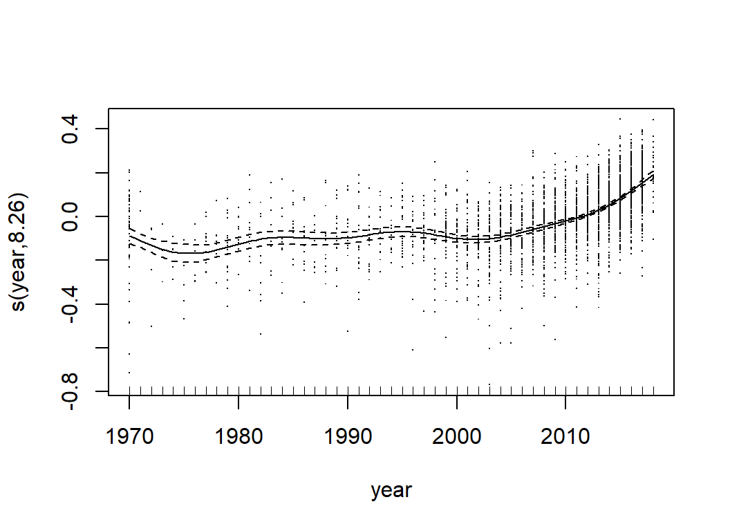
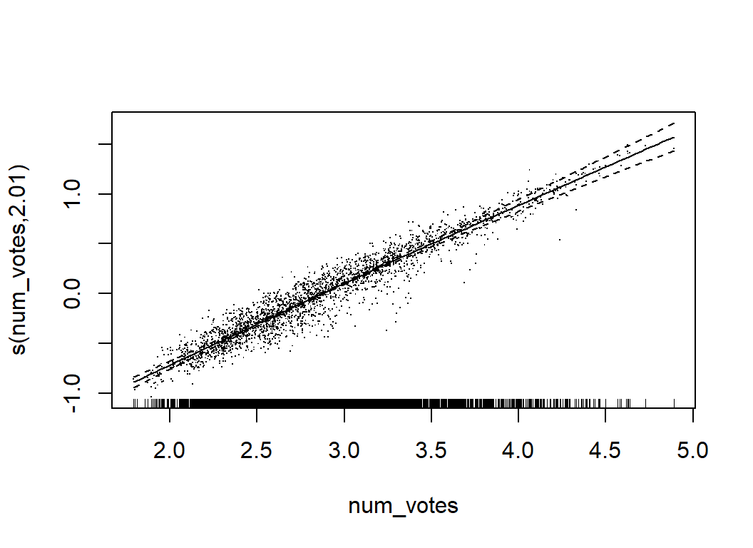
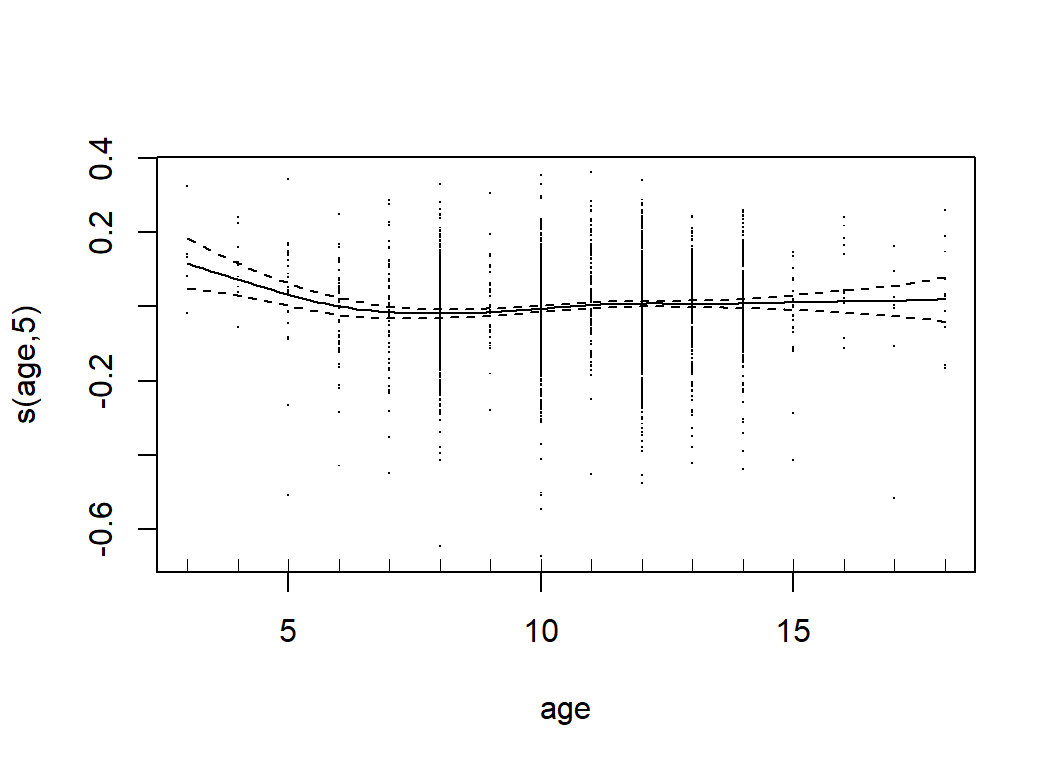
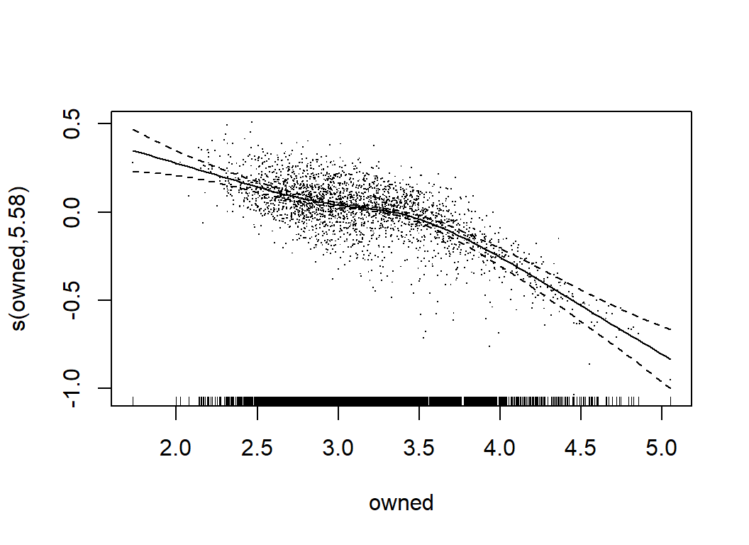
GAMs are much more flexible than simple linear models, but they are still relatively easy to interpret. We can tell what features are most important and we can describe the relationships between the predictors and the response. Their main limitation is that GAMs do not readily incorporate interactions. When the form of an interaction is known, it can be incorporated ‘by hand’, but the possible forms of interaction are so wide ranging that an automatic method is almost essential.
mgcv does include higher dimensional splines, so we might try predicting geek_rating from a two-dimensional spline function over, say, num_votes and owned but there is a problem. Suppose that we were to place a two dimensional spline over year and log10(avg_time); one variable will have a range of over 50 while the other’s range will be in single digits. The scale affects the size of the regression coefficients and the optimum smoothness penalty depends on those coefficients. So year and log10(avg_time) will require different sized penalties for the same degree of wiggliness. When they are combined in a 2-dimensional spline, it may be impossible to find penalty that works in both dimensions. There are two possible solutions; scale the variables so that they have similar ranges or use tensor product splines that are scale invariant. I’ve opted for the former though mgcv will fit tensor product splines, if you want them.
We know that owned and num_votes are key variables that are highly correlated, so I will try including their interaction. I should imagine that young children would prefer shorter games, so I will add a avg_time by age interaction and I suspect that more recent games might get more votes, so I’ll add a year by num_votes interaction. You could, of course, be more systematic and try all two feature interactions in turn.
When you have main effects and interactions in the same model there is a degree of over-parameterisation. In mgcv you can control this yourself, but I have been lazy and left it to the package to sort it out.
Before running the analysis, the predictors must be scaled. I already have trainDF but I want to scale testDF and trainDF in the same way, so I’ll need to start by creating testDF.
# --- create testDF --------------------------------------------
readRDS( file.path(home, "data/rData/clean_test.rds")) %>%
  mutate( owned       = log10(owned),
          num_votes   = log10(num_votes),
          min_players = log10(min_players),
          max_players = log10(max_players),
          min_time    = log10(min_time),
          max_time    = log10(max_time),
          avg_time    = log10(avg_time)) -> testDF

# --- standardise both training and test data -------------------
for( v in c("owned", "num_votes", "min_players", "max_players",
           "min_time", "max_time", "avg_time", "year", "age") ) {
  m <- mean(trainDF[[v]])
  s <- sd(trainDF[[v]])
  trainDF[[v]] <- (trainDF[[v]] - m)/s
  testDF[[v]]  <- (testDF[[v]]  - m)/s
  }

# --- split the data as before ----------------------------------
validateDF <- trainDF[  split, ]
estimateDF <- trainDF[ -split, ]
Now we can fit an interaction model
# --- refit the no interaction GAM ----------------------------------
estimateDF %>%
  { gam( geek_rating ~ s(max_players) + s(avg_time) +
           s(year) + s(num_votes) + s(age) + s(owned) +
           M1 + M8 + M9 + M10 +
           C1 + C2    , data=.) } -> mod0

# --- fit a GAM with interaction -------------------------------------
estimateDF %>%
  { gam( geek_rating ~ s(max_players) + s(avg_time) +
           s(year) + s(num_votes) + s(age) + s(owned) +
           s(num_votes, owned) + s(avg_time, age) + s(year, num_votes) +
           M1 + M8 + M9 + M10 +
           C1 + C2    , data=.) } -> mod

# --- RMSE -----------------------------------------------------------
metrics(mod)
## Estimation RMSE: 0.160
## Validation RMSE: 0.173# --- Analysis of Variance -------------------------------------------
anova(mod0, mod)## Analysis of Deviance Table
##
## Model 1: geek_rating ~ s(max_players) + s(avg_time) + s(year) + s(num_votes) +
## s(age) + s(owned) + M1 + M8 + M9 + M10 + C1 + C2
## Model 2: geek_rating ~ s(max_players) + s(avg_time) + s(year) + s(num_votes) +
## s(age) + s(owned) + s(num_votes, owned) + s(avg_time, age) +
## s(year, num_votes) + M1 + M8 + M9 + M10 + C1 + C2
## Resid. Df Resid. Dev Df Deviance
## 1 2456.1 38.322
## 2 2399.2 34.246 56.867 4.0756Only a slight improvement in the RMSE of the validation sample to 0.173 and the interactions need over 50 degrees of freedom to reduce the deviance by 4. They really are not worth it.
Whether or you go beyond this GAM model depends on your aims. In the real world, small gains in the precision of the predictions are likely to be less important than the development of understanding of the structure of the data, but these data were presented for a competition, so this is not the real world.
Submission
I opt to use the GAM with selected features and no interactions. So let’s prepare a submission. I’ll fit the GAM to the full set of clean training data and then predict for the test data.
Here is the format of the sample submission that we need to copy.
read_csv( file.path(home, "data/rawData/sample_submission.csv") ) %>%
  print()
## # A tibble: 1,500 x 2
## game_id geek_rating
## <dbl> <dbl>
## 1 174430 6.09
## 2 182028 6.09
## 3 12333 6.09
## 4 180263 6.09
## 5 84876 6.09
## 6 173346 6.09
## 7 115746 6.09
## 8 102794 6.09
## 9 96848 6.09
## 10 183394 6.09
## # ... with 1,490 more rows# --- fit the GAM to the full training set ---------------------------
trainDF %>%
{ gam( geek_rating ~ s(max_players) + s(avg_time) +
s(year) + s(num_votes) + s(age) + s(owned) +
M1 + M8 + M9 + M10 +
C1 + C2 , data=.) } -> mod
# --- predict and write to csv ---------------------------------------
testDF %>%
mutate( .fitted = predict(mod, newdata=. ) ) %>%
mutate( geek_rating = 5.5 + 10^.fitted ) %>%
select( game_id, geek_rating) %>%
print() %>%
write_csv( file.path(home, "temp/submission1.csv") )## # A tibble: 1,500 x 2
## game_id geek_rating
## <dbl> <dbl>
## 1 174430 7.86
## 2 182028 8.30
## 3 12333 7.97
## 4 180263 7.80
## 5 84876 7.42
## 6 173346 7.79
## 7 115746 7.28
## 8 102794 7.80
## 9 96848 7.85
## 10 183394 7.43
## # ... with 1,490 more rowsI submitted this file as a ‘late submission’ to https://www.kaggle.com/c/sliced-s01e01/.
On the private leaderboard there is one submission that scored 0.026. It is so much better than all of the others that it is suspicious (it would be possible to download the ratings from the BGG website). If it is genuine, then I would very much like to see the model that was used. The next best score is 0.161 and I take this to be the true benchmark.
The GAM model scored 0.169 on the private leaderboard. As expected, the validation score gives a good indication of the performance in the test set. This GAM would have finished in 5th place. To do better, I would need to make a more systematic investigation of interactions and perhaps look at more text features.
What this example shows
This is a great example to have chosen for the first episode. There is enough in it to create a real challenge for the contestants and yet it is not so complex that they would be overwhelmed.
One of the topics that interests me is the relationship between statistical analysis and data science. People who want to stress the differences often point to specific algorithms, but I think that this is a mistake. There are no machine learning algorithms that would not fit neatly into a statistics course, indeed many of the most commonly used algorithms were first suggested by statisticians.
I think that the differences between statistics and data science are quite minor, but one place where they do vary is in their objectives. Statisticians usually use models in order to discover relationships or test hypotheses that will apply beyond the current data set, that is to say they are primarily interested in findings that will generalise. In contrast, machine learning is more likely to be concerned with the actual data that are being analysed.
This difference in emphasis does not change the models, but it does affect the ways in which those models are judged. Generally, machine learning leans towards models that represent the fine structure of the training data, while statisticians tend to choose models that capture its broader structure.
I hope that my analysis has shown that linear models are competitive with the more fashionable tree-based algorithms favoured by most competitors. My model is not top of the leaderboard, but the the difference between the GAM’s RMSE and the leader’s is slight and had the organisers used a different seed for the random number generator when they split the test data from the training data, it is possible that the order would have been reversed. In my opinion the difference between RMSEs of 0.161 and 0.169 is meaningless. I am more interested in the ease of interpretation of the GAM and its generalisability.
It seems to me that the emphasis on data visualisation in Sliced and in data science in general is in part driven by the fact that they choose models that are difficult to interpret.
Why do statisticians put so much store on interpretation of the model? Obviously, the results from a model that has meaning are easier to communicate to others, but there are other reasons. Interpretable models help in the modelling cycle, as understanding the results will help the analyst suggest ways of improving the model. Equally important, when an analyst uses a model that can be interpreted, they are far less likely to do something stupid. Modelling is complex and everyone makes errors, but there is a much better chance that the mistake will be spotted if the model fit has meaning.
Machine learning algorithms are usually tested by random splitting. The organisers of Sliced split the data from the website into a training set and a test set, I split the training data into an estimation set and a validation set and mgcv used cross-validation on the estimation set in order to select the smoothness of the splines.
Random splitting produces two very similar sets of data, so similar that all that the test set does, is provide an unbiased estimate of the model’s performance in the training set. Randomly sampled test data tells us nothing about the world beyond the current set of training data. RFor instance, random splitting says nothing about questions such as, will the model still be predictive on next year’s data? if BGG were to create a Spanish language website and they collected user data in an identical way, would the structure of the model still be applicable?
Perhaps, occasionally, Sliced should set a broader objective. For this episode, they could have withheld the data for games released after the start of 2018 and set the task of creating a model using pre-2018 data. I suspect that GAMs would perform better than boosted trees in such a competition, because boosted trees are more likely to follow blips in the data. The blips are actually present in the training data, so they will be duplicated when the data are split at random, but they may well not be seen in an independently collected data set.
Appendix
Here are the functions used in the analysis of the text. Obtaining features from text is a common preprocessing task and there are packages such as tidytext and quanteda that will do this for us. I’ll make a point of using some of those packages in the future, but for now I have just used my own functions.
# --- select_indicators() ------------------------------------------
# a function to automate the selection of comma delimited text items
#   thisDF   ... the data frame containing the data
#   col      ... the column containing the text
#   response ... the field used to indicate difference
#   nTerms   ... max number of text items to extract from a column
#   minCount ... smallest frequency of a selected item
#   sep      ... separator used to divide col
# return
#   a tibble of selected items, their frequency, a t-test p-value and
#   mean geek_rating when text item is present/absent
#
select_indicators <- function(thisDF, col, response,
                              nTerms=5, minCount=25, sep=",") {
  # --- make a vector of common terms --------------------------------
  thisDF %>%
    select({{col}}) %>%
    separate({{col}}, sep=sep,
             into=paste("x", 1:nTerms, sep=""),
             remove=TRUE, extra="drop", fill="right" ) %>%
    pivot_longer(everything(), values_to="terms", names_to="source" ) %>%
    filter( !is.na(terms) ) %>%
    mutate( terms = str_trim(terms)) %>%
    filter( terms != "" ) %>%
    group_by( terms) %>%
    summarise( n = n() , .groups="drop") %>%
    arrange( desc(n)) %>%
    filter( n >= minCount ) %>%
    pull( terms ) -> tVec

  # --- how many possible items -------------------------
  n <- length(tVec)
  # --- Tibble for the results --------------------------
  tibble( term     = tVec,
          count    = integer(n),
          p_value  = double(n),
          mWithout    = double(n),
          mWith    = double(n)) -> resDF
  # --- perform n t-tests -------------------------------
  for( i in 1:n ) {
    thisDF %>%
      mutate( y = {{response}} ) %>%
      mutate( class = as.numeric(str_detect({{col}}, tVec[i]))) %>%
      filter( !is.na(class) ) -> tDF
    if( max(tDF$class) != 1 | min(tDF$class != 0)) {
      resDF$p_value[i] <- NA
    } else {
      resDF$p_value[i] <- t.test(tDF$y ~ tDF$class )$p.value
    }
    resDF$count[i]   <- sum(tDF$class == 1)
    resDF$mWithout[i]   <- mean(tDF$y[tDF$class==0])
    resDF$mWith[i]   <- mean(tDF$y[tDF$class==1])
  }
  # --- sort and return --------------------------------
  resDF %>%
    arrange(p_value) %>%
    return()
}

# --- make_indicators() ------------------------------------------------
# a function to make indicator variables from text items
#   col      ... vector containing the text
#   targets  ... vector of text items to use
#   prefix   ... if prefix="x", indicators are "x1", "x2", ...
# return
#   a tibble of indicator variables
#
make_indicators <- function(col, targets, prefix="x") {
  L <- as.list(targets)
  names(L) <- paste(prefix, 1:length(targets), sep="")
  map_df(L, ~ as.numeric(str_detect(col, .x)) ) %>%
    return()
}

# --- add_indicators() ------------------------------------------------
# a function to combine indicators variable in a tibble
#   thisDF   ... the data frame to which the indicators are added
#   col      ... name of column containing the text
#   targets  ... vector of text items to use
#   prefix   ... if prefix="x", indicators are "x1", "x2", ...
# return
#   a tibble with added indicator variables
#
add_indicators <- function(thisDF, col, targets, prefix="x") {
  cbind( thisDF,
         make_indicators(thisDF[[col]], targets, prefix) ) %>%
    as_tibble()
}