Introduction

The fundamental idea that underpins all machine learning is that of the universal approximator, that is, a function that is so flexible that it can be used to model any dataset. Trees provide one way to construct such a flexible function.

The code below simulates a small regression problem that I will use to illustrate the discussion of Bayesian tree models.

# --- create an example dataset ------------------------------
set.seed(8920)
tibble( x1 = rnorm(400, 0, 1),
        x2 = runif(400, 0, 1),
        y  = 10 - (x1 - 1)^2 + 10 * x2 - 
          x1 * log(x2) + rnorm(400, 0, 0.25)) -> trainDF

# --- plot y vs x1 and y vs x2 -------------------------------
library(patchwork)
trainDF %>%
  ggplot( aes(x=x1, y=y)) +
  geom_point() -> p1

trainDF %>%
  ggplot( aes(x=x2, y=y)) +
  geom_point() -> p2

p1 + p2 +
  plot_annotation(title="Response, y, and two predictors, x1 and x2.")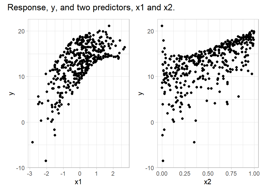

The formula for generating y shows that a model that was able to capture the trend exactly would make predictions with a RMSE of 0.25. However, the scatter plots suggest that it will not be easy to approximate that trend.

Here is a linear regression model fitted to these data.

library(broom)
trainDF %>%
  lm( y ~ x1 + x2, data = . ) %>%
  {
    tidy(.) %>% print()
    glance(.) %>% print()
  }

## # A tibble: 3 × 5
##   term        estimate std.error statistic   p.value
##   <chr>          <dbl>     <dbl>     <dbl>     <dbl>
## 1 (Intercept)     8.20    0.171       48.0 2.64e-167
## 2 x1              2.99    0.0856      34.9 3.47e-123
## 3 x2              9.60    0.299       32.1 1.79e-112
## # A tibble: 1 × 12
##   r.squared adj.r.squ…¹ sigma stati…²   p.value    df logLik   AIC   BIC devia…³
##       <dbl>       <dbl> <dbl>   <dbl>     <dbl> <dbl>  <dbl> <dbl> <dbl>   <dbl>
## 1     0.844       0.844  1.75   1077. 4.16e-161     2  -790. 1589. 1605.   1218.
## # … with 2 more variables: df.residual <int>, nobs <int>, and abbreviated
## #   variable names ¹​adj.r.squared, ²​statistic, ³​deviance

The residual standard deviation (sigma) is 1.75, a long way from what is theoretically possible.

A tree-based regression model approximates the trend by a series of horizontal lines. For ease of representation, I will picture a tree that predicts y from x2 alone. I split the x2 scale into three regions using thresholds at 0.3 and 0.7 and then predict y by the mean of the observed y’s within each of the regions.

# --- summary statistics for each region -----------------------
trainDF %>%
  mutate( region = 1 + (x2 > 0.3) + (x2 > 0.7)) %>%
  group_by(region) %>%
  summarise( n = n(),
             m = mean(y),
             s = sd(y)) %>%
  print() -> predDF

## # A tibble: 3 × 4
##   region     n     m     s
##    <dbl> <int> <dbl> <dbl>
## 1      1   130  9.88  4.42
## 2      2   150 13.2   3.32
## 3      3   120 16.2   3.11

# --- residual standard deviation for this tree ----------------
trainDF %>%
  mutate( region = 1 + (x2 > 0.3) + (x2 > 0.7)) %>%
  group_by(region) %>%
  mutate( m = mean(y)) %>%
  ungroup() %>%
  summarise( rmse = sqrt( mean( (y - m)^2 ) ) )

## # A tibble: 1 × 1
##    rmse
##   <dbl>
## 1  3.64

A RMSE of 3.64 is even worse than linear regression, but one can imagine improving performance by using more cut points and by making use of x1.

This type of model can be pictured in one of two ways. The first is by superimposing the regions on the scatter plot of y on x2.

# --- regions of x2 and the corresponding mean estimates ------------------
trainDF %>%
  ggplot( aes(x=x2, y=y)) +
  geom_point() +
  geom_vline( xintercept = c(0.3, 0.7), linetype=2, colour="red") +
  geom_segment( aes( x=0, y=9.88, xend=0.3, yend=9.88), colour="blue", size=2) +
  geom_segment( aes( x=0.3, y=13.2, xend=0.7, yend=13.2), colour="blue", size=2) +
  geom_segment( aes( x=0.7, y=16.2, xend=1, yend=16.2), colour="blue", size=2) +
  labs( title = "Regions and their predictions")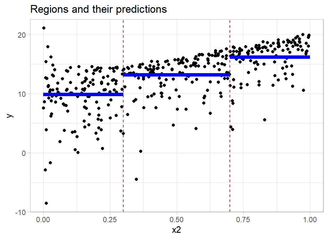

The second representation is as a binary decision tree in which answering no to a question leads to the left branch and answering yes leads to the right branch. mu is my symbol for the prediction.

library(DiagrammeR)

mermaid("
graph TB
  A(root)-->B(x2>0.3)
  B-->C(mu=9.88)
  B-->D(x2>0.7)
  D-->E(mu=13.2)
  D-->F(mu=16.2)
")

A non-Bayesian would search for the optimal tree by defining a loss function, probably the RMSE. Then, using a guided form of trial and error, they would search over the space of possible trees until they found the one that minimises the loss. There are computational issues and questions about when to stop, but this idea is the basis of the method called CART that is implemented in the R package rpart.

A Bayesian looks at the problem rather differently. They formulate the problem in terms of probability, so they need a model for the y values in the jth terminal node, perhaps N(\(\mu_j\), \(\sigma\)). Given a particular tree, they can use this distribution to calculate the likelihood of the data, that is, P(Data|Model). Then, by placing priors on the tree structure and on the node parameters, this likelihood can be inverted by Bayes theorem to produce P(Model|Data). In other words, every tree has a probability. A Bayesian algorithm searches for a sample of trees that have high probability.

The key difference between the loss function and the Bayesian approaches is that the former provides a single best fitting tree, while the latter provides a set of trees that reflect our uncertainty about the true model.

Sum of trees

A single tree provides a slightly crude model in that every observation that falls in the same terminal node will get exactly the same prediction. An obvious extension is to use a collection of trees, so that observations that fall in the same terminal node of one tree might be split apart in another tree. The final prediction is set equal to the sum of the contributions from the different trees, which provides a finer resolution.

Bayesian sums of trees regression models were first proposed in the late 1990s and they are still the subject of much research. The idea was presented in a technical report and later published as,

Chipman, H., George, E., & McCulloch, R. Bayesian ensemble learning.
Advances in neural information processing systems, (2006) 19.

The BART (Bayesian Additive Regression Trees) model combines H trees, labelled h=1…H, each with its own set of terminal node parameters. The contribution to the sum from predictors that fall in the jth terminal node of tree h is, \[ \mu_{hj} \sim N(0, \sigma_\mu) \] The set of \(\mu\)’s for tree, \(T_h\), is called \(M_h\) and the function that picks out the appropriate \(\mu\) given predictors x is \(g(x; T_h, M_h)\).

Under the model, the ith observation, \(y_i\), is assumed to be normally distributed, \[ y_i \sim \text{N} \left( \sum_{h=1}^H g(x_i; T_h, M_h), \ \ \sigma \right) \] So \(\sigma\) measures the inherent variability of the response about its trend (0.25 in our example) and \(\sigma_\mu\) measures the variability of the contributions from the different terminal nodes. These standard deviations are assumed constant over all nodes and all observations.

R Packages for Bayesian tree models

In R, there are four packages that implement this algorithm, BayesTree, dbarts, bartMachine and BART.

The BayesTree package implements the methods described in

Chipman, H., George, E., and McCulloch R.
Bayesian Additive Regression Trees.
The Annals of Applied Statistics, 2010, 4,1, 266-298.

Unfortunately, the BayesTree implementation in R is too slow for practical use. Two early attempts were made to speed the computation. bartMachine written in Java and run via the rJava package and dbarts written in C++ and accessed directly from R. In my limited experience, the Java version is the quicker, but it leaves the results in a Java object, which means that you either have to unpick that object yourself, or you are reliant on the functions provided in the package. dbarts is essentially a fast copy of BayesTree, but it is designed so that it could be incorporated into a more general user-written sampler.

The most recent offering is the package BART, which is written in C++ and which has comparable speed to dbarts and bartMacine. Its big advantage is that it offers versions of the algorithm for different types of response, including binary, categorical, time to event and it incorporates variable selection. The package is described in

Sparapani, Rodney, Charles Spanbauer, and Robert McCulloch.
Nonparametric machine learning and efficient computation with bayesian additive regression trees: the BART R package.
Journal of Statistical Software 97.1 (2021): 1-66.

This paper includes a useful table comparing the features available in each of the four packages. I have tried all four and in my opinion, BART is the best option.

Analysis with BART

I will take the toy example and analyse it with BART to illustrate how the package is used. To complete the example, I first create a set of test data generated under the same model as trainDF.

# --- create a test dataset ------------------------------
set.seed(5504)
tibble( x1 = rnorm(200, 0, 1),
        x2 = runif(200, 0, 1),
        y  = 10 - (x1 - 1)^2 + 10 * x2 - 
          x1 * log(x2) + rnorm(200, 0, 0.25)) -> testDF

BART requires the data in vectors and matrices, so I create them.

library(BART)

# --- extract training Y into a vector --------------------
trainDF %>%
  pull(y) -> Y

# --- extract training predictors into a matrix -----------
trainDF %>%
  select(x1, x2) %>%
  as.matrix() -> X


# --- extract test Y into a vector ------------------------
testDF %>%
  pull(y) -> YT
  

# --- extract test predictors into a matrix ---------------
testDF %>%
  select(x1, x2) %>%
  as.matrix() -> XT

First, I analyse the example by running three default chains using wbart(); this is the BART function for modelling continuous responses.

I have written a simple function, reportBart(), that prints performance indicators. The code is given in an appendix at the end of this post.

# --- default sum of trees: run 3 times --------------------
set.seed(8987)
bt1 <- wbart(x.train = X, y.train = Y, x.test = XT)
reportBart(bt1, Y, YT, thin=1)
set.seed(3456)
bt2 <- wbart(x.train = X, y.train = Y, x.test = XT) 
reportBart(bt2, Y, YT, thin=1)
set.seed(2098)
bt3 <- wbart(x.train = X, y.train = Y, x.test = XT) 
reportBart(bt3, Y, YT, thin=1)

## 200  trees: run length  1000  burn-in  100  thin by  1 
##  Posterior mean sigma     0.2804047 
##  Average splits per tree  1.262235 
##  training RMSE            0.1900273 
##  test RMSE                0.431628

## 200  trees: run length  1000  burn-in  100  thin by  1 
##  Posterior mean sigma     0.2925698 
##  Average splits per tree  1.257975 
##  training RMSE            0.1989069 
##  test RMSE                0.4902702

## 200  trees: run length  1000  burn-in  100  thin by  1 
##  Posterior mean sigma     0.2805821 
##  Average splits per tree  1.232065 
##  training RMSE            0.1920744 
##  test RMSE                0.4391365

The computation took around 2s per chain. BART’s default is to sum over 200 trees using a chain of length 1000 after a burn-in of 100. My summary tables show that the trees are not very deep, they are based on average of about 1.2 splits per tree and the model seems to be over-fitting. The RMSE for the training data is much lower than that for the test data.

The algorithm estimates two parameters; the residual standard deviation, sigma, and the sum of tree contributions for each observation, \(\sum g(x_i; T_h, M_h)\).

It is important to check for convergence of the algorithm and the simplest starting point is the convergence of sigma. I use the trace plotting function, trace_plot(), described in my previous Bayesian methods posts.

library(MyPackage)

# --- pack sigma estimates into a tibble ------------------
tibble(sigma = c(bt1$sigma, bt2$sigma, bt3$sigma),
       iter  = rep(1:length(bt1$sigma), times=3),
       chain = rep(1:3, each=length(bt1$sigma))) %>%
  # --- drop burn-in ------------------
  filter( iter > 100 ) -> simDF

# --- trace plots of sigma --------------------------------
simDF %>%
  trace_plot( sigma )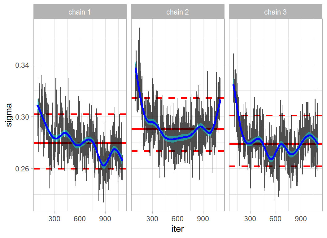

Mixing is not great and the three chains are not really in agreement. After a little trial and error, I decided on a burn-in of 5000 and a run of length 20,000 from which I saved every 20th iteration. Each of these chains takes 41s to run on my desktop.

# --- sum of trees: longer chains -------------------------
set.seed(8987)
bt4 <- wbart(x.train = X, y.train = Y, x.test = XT,
             nskip=5000, ndpost = 1000, keepevery = 20) 
reportBart(bt4, Y, YT, thin=20)
set.seed(3456)
bt5 <- wbart(x.train = X, y.train = Y, x.test = XT,
             nskip=5000, ndpost = 1000, keepevery = 20) 
reportBart(bt5, Y, YT, thin=20)
set.seed(2098)
bt6 <- wbart(x.train = X, y.train = Y, x.test = XT,
             nskip=5000, ndpost = 1000, keepevery = 20) 
reportBart(bt6, Y, YT, thin=20)

## 200  trees: run length  1000  burn-in  5000  thin by  20 
##  Posterior mean sigma     0.2654372 
##  Average splits per tree  1.20304 
##  training RMSE            0.168509 
##  test RMSE                0.4317386

## 200  trees: run length  1000  burn-in  5000  thin by  20 
##  Posterior mean sigma     0.2632656 
##  Average splits per tree  1.181055 
##  training RMSE            0.1664701 
##  test RMSE                0.4188793

## 200  trees: run length  1000  burn-in  5000  thin by  20 
##  Posterior mean sigma     0.2637268 
##  Average splits per tree  1.187155 
##  training RMSE            0.1687145 
##  test RMSE                0.3821009

The trace plot for sigma is much better (code hidden as it is essentially the same as that used before).

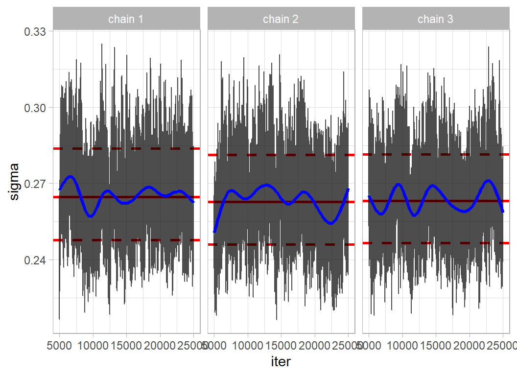
Pooling the 3 chains allows us to visualise the posterior.

simDF %>%
  summarise( m = mean(sigma),
             lb = quantile(sigma, probs=0.025),
             ub = quantile(sigma, probs=0.975) ) %>%
  print() -> statDF

## # A tibble: 1 × 3
##       m    lb    ub
##   <dbl> <dbl> <dbl>
## 1 0.264 0.238 0.293

simDF %>%
  ggplot( aes(x=sigma)) +
  geom_density( fill="steelblue") +
  geom_vline( xintercept = c(statDF$m, statDF$lb, statDF$ub),
                 linetype = c(1,2,2), colour="red") +
  labs(title="Posterior distribution of sigma",
       subtitle = "Showing the posterior mean and 95% CrI")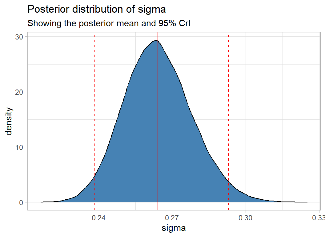

BART also returns the predictions for each of the 400 training data points after each of the 1000 iterations. They are placed in a 1000x400 matrix called yhat.train.

I combine these estimates and then, for illustration, look at the convergence of the prediction corresponding to the first observation.

# --- predictions for each training observation
rbind(bt4$yhat.train, bt5$yhat.train, bt6$yhat.train)  %>%
  as_tibble() %>%
  mutate(iter  = rep(1:1000, times=3),
         chain = rep(1:3, each=1000))  -> predDF

# --- trace plot of predictions for observation 1
predDF %>%
  trace_plot(V1) +
  geom_hline(yintercept=Y[1], size=1.5, colour="darkgreen") +
  labs( y = "Observation 1",
        title = "trace plot of prediction for observation 1",
        subtitle = "Actual value shown in green")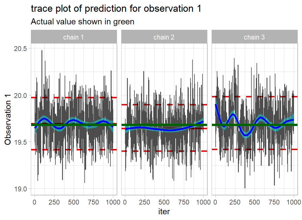

Convergence is ball-park OK, but far from perfect.

For more detailed convergence checking the estimates can be coerced into mcmc objects for use in coda. Below, I look at the predictions for the first 100 observations and calculate the Rhat statistics that compare variances within and between chains.

library(coda)

# --- predictions for the first 100 observations -----------
mc <- mcmc.list(
        mcmc(bt4$yhat.train[,1:100]), 
        mcmc(bt5$yhat.train[,1:100]), 
        mcmc(bt6$yhat.train[,1:100]))

# --- gelman statistic Rhat --------------------------------
gd <- gelman.diag(mc)

# --- Rhat in descending order
gd$psrf %>%
  as_tibble() %>%
  janitor::clean_names("lower_camel") %>%
  mutate( observation = paste0("V", 1:100)) %>%
  select( observation, everything() ) %>%
  arrange( desc(pointEst) )

## # A tibble: 100 × 3
##    observation pointEst upperCI
##    <chr>          <dbl>   <dbl>
##  1 V88             1.27    1.73
##  2 V25             1.14    1.41
##  3 V81             1.11    1.33
##  4 V48             1.11    1.32
##  5 V100            1.10    1.31
##  6 V31             1.10    1.30
##  7 V95             1.09    1.30
##  8 V96             1.09    1.28
##  9 V42             1.09    1.27
## 10 V80             1.08    1.24
## # … with 90 more rows

Ideally, Rhat should be 1.0 and there was a time when a point estimate of 1.2 was considered close enough to 1, but today, researchers typically require values below 1.05 (see my methods post on assessing convergence). Observation 88 is highlighted as having poor convergence, so below I plot its trace.

# --- trace plot of Observation 88 selected because of its high Rhat
predDF %>%
  trace_plot(V88) +
  geom_hline(yintercept=Y[88], size=1.5, colour="darkgreen") +
  labs( y = "Observation 88",
        title = "trace plot of predictions for observation 88",
        subtitle = "Actual value shown in green")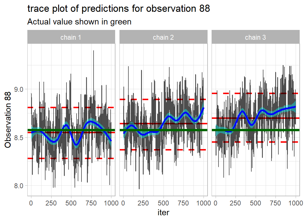

The chains are still drifting and the chains have different means.

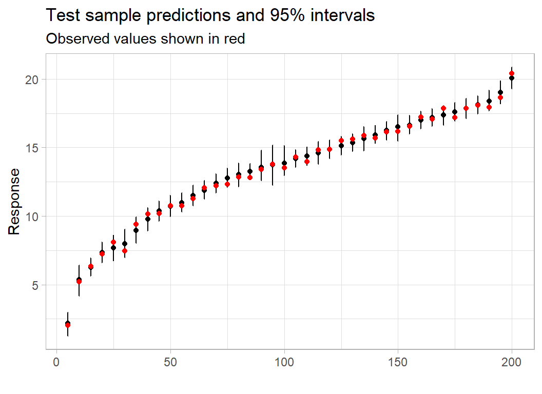
Although, the convergence is not really good enough, I’ll continue to look at the quality of the predictions. In the next plot, I reorder the observations and compare them with their posterior mean prediction and an approximate 95% CrI for the value y. To create the CrI for y rather than for the prediction I add a normal random error with standard deviation, sigma. The value of sigma should itself be randomly chosen from the posterior of sigma, but for simplicity I have used the posterior mean.

# --- predictions + a random error term
rbind(bt4$yhat.train, bt5$yhat.train, bt6$yhat.train) +
  matrix( rnorm(1200000, 0 , 0.264 ), nrow=3000, ncol=400)  %>%
  as_tibble() %>%
  mutate(iter  = rep(1:1000, times=3),
         chain = rep(1:3, each=1000))  -> predDF

# --- summary statistics for the 400 predictions --------------
predDF %>%
  summarise( across(starts_with("V"), 
                    list(mean, sd,
                         ~ quantile(.x, probs=0.025), 
                         ~ quantile(.x, probs=0.975)))) %>%
  pivot_longer(everything(), names_to="v", values_to="stat") %>%
  separate( v, into=c("obs", "j"), sep="_") %>%
  pivot_wider(names_from=j, values_from=stat) %>%
  rename( m = `1`, sd = `2`, q1 = `3`, q2 = `4`) %>%
  mutate( obs = str_replace(obs, "V", "Y")) %>%
  mutate( y = Y)  -> statDF

# --- plot every 5th prediction -------------------------------
statDF %>%
  arrange(m) %>%
  mutate( x = row_number()) %>%
  filter( x %% 5 == 0 ) %>%
  ggplot( aes(x= x, y=m)) +
  geom_point() +
  geom_errorbar( aes(ymin=q1, ymax=q2), width=0.2) +
  geom_point( aes(x=x, y=y), colour="red") +
  labs( y = "Response", x = "",
  title = "In-sample predictions and 95% intervals",
  subtitle = "Observed values shown in red")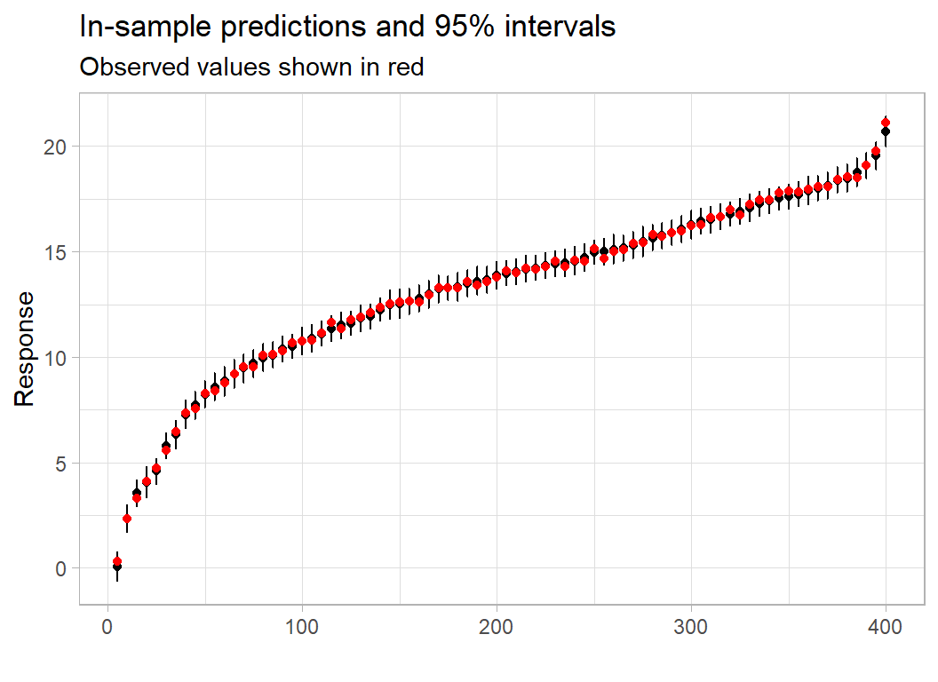

These credible intervals express our uncertainty about the observations y. It looks as though the observations are too close to the posterior mean predictions, suggesting that the model is over-fitting.

Bayesian measures of surprise can be used to identify the observations that are poorly predicted.

# --- residuals as a measure of surprise ------------------
statDF %>%
  mutate( r = (y-m)/sd ) %>%
  arrange(r) %>%
  {
    head(.) %>% print()
    tail(.) %>% print()
  }

## # A tibble: 6 × 7
##   obs       m    sd    q1    q2     y      r
##   <chr> <dbl> <dbl> <dbl> <dbl> <dbl>  <dbl>
## 1 Y293   15.1 0.301  14.5  15.7  14.6 -1.73 
## 2 Y134   15.9 0.311  15.3  16.5  15.4 -1.71 
## 3 Y2     15.7 0.317  15.1  16.3  15.2 -1.47 
## 4 Y138   11.4 0.303  10.8  12.0  11.0 -1.22 
## 5 Y167   15.4 0.303  14.8  16.0  15.0 -1.04 
## 6 Y140   17.5 0.329  16.9  18.2  17.2 -0.982
## # A tibble: 6 × 7
##   obs       m    sd    q1    q2     y     r
##   <chr> <dbl> <dbl> <dbl> <dbl> <dbl> <dbl>
## 1 Y51    18.2 0.324  17.6  18.9  18.6  1.17
## 2 Y349   15.0 0.323  14.4  15.6  15.4  1.21
## 3 Y94    18.4 0.312  17.8  19.0  18.8  1.30
## 4 Y354   14.0 0.317  13.4  14.6  14.4  1.31
## 5 Y360   18.3 0.297  17.7  18.9  18.8  1.63
## 6 Y5     16.5 0.308  15.9  17.1  17.2  2.37

Overall in-sample prediction looks good, perhaps too good.

Next, I make the prediction plot for the test data. The code is so similar that I will not show it.

Another matrix returned by BART is varcount, it represents the total number of times that each predictor is used to split a tree (summed over the 200 trees) and provides a measure of variable importance. The count is given for each iteration of the sampler.

The plot shows varcount for the first of my longer runs.

# --- average number of splits -----------------------------
bt4$varcount %>%
  as_tibble() %>%
  ggplot( aes(x=1:1000, y=x1 /200) ) +
  geom_line( colour="red") +
  geom_line( aes(x=1:1000, y=x2 / 200), colour="blue" ) +
  geom_line( aes(x=1:1000, y=(x1+x2) / 200), colour="darkgreen" ) +
  labs( x = "Iteration",
        y = "Splits",
        title = "Average number of splits per tree")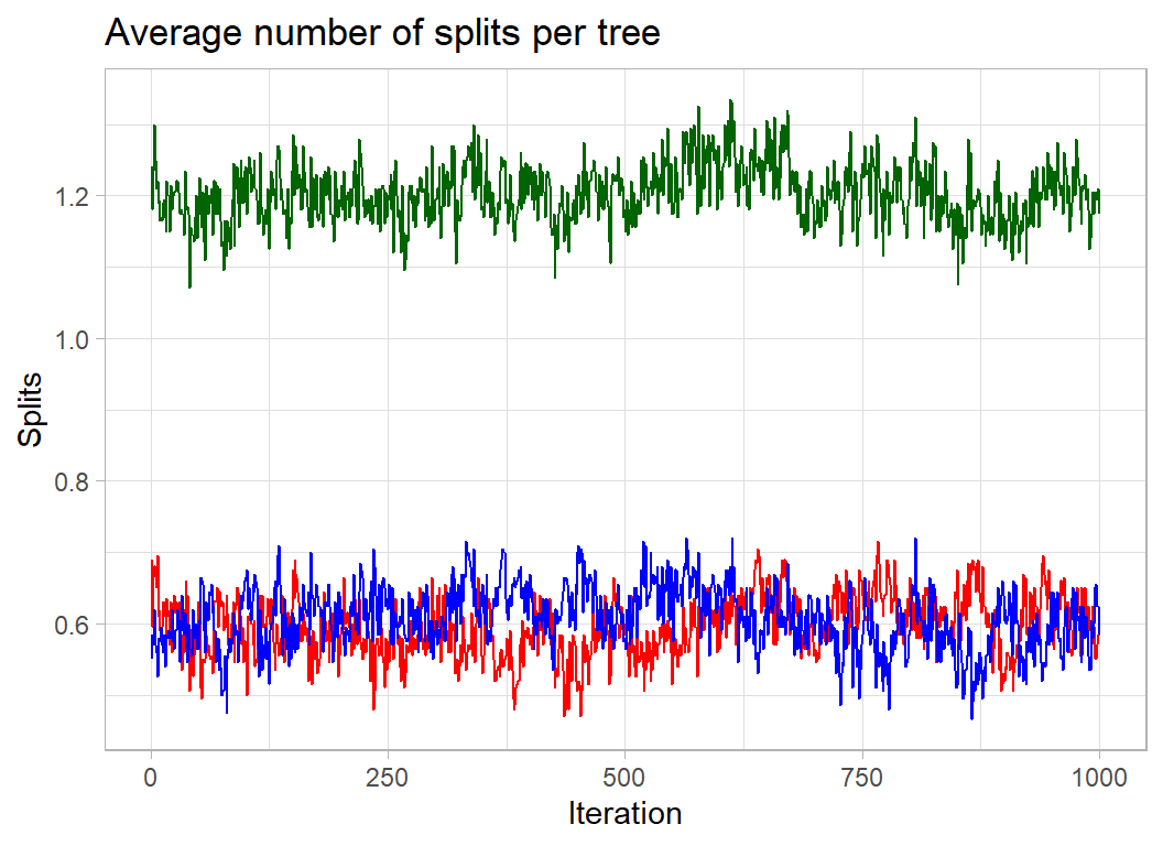

We can see that x1 and x2 are used equally often and that the trees have on average only 1.2 splits; they very stumpy. As intended, the algorithm gets its performance by averaging a set of weak learners.

Varying the number of trees

The priors have a regularising effect on the model, but the final form will owe much more to the data than to those priors. The defaults lead to sensible models for most datasets, however there is one hyperparameter than can make a difference; the number of trees. The BayesTree package set the default number of trees to 50, while BART has changed this to 200. At first sight, it might seem that summing over 200 trees is bound to give better predictions than summing over 50 trees, but this is not guaranteed.

# --- sum of 50 trees ------------------------
set.seed(8987)
bt7 <- wbart(x.train = X, y.train = Y, x.test = XT, ntree=50, nskip=5000, ndpost = 1000, keepevery = 20) 

The performance measures are,

# --- with 200 trees
reportBart(bt4, Y, YT, thin=20)

## 200  trees: run length  1000  burn-in  5000  thin by  20 
##  Posterior mean sigma     0.2654372 
##  Average splits per tree  1.20304 
##  training RMSE            0.168509 
##  test RMSE                0.4317386

# --- with 50 trees
reportBart(bt7, Y, YT, thin=20)

## 50  trees: run length  1000  burn-in  5000  thin by  20 
##  Posterior mean sigma     0.296641 
##  Average splits per tree  1.55248 
##  training RMSE            0.2114193 
##  test RMSE                0.596489

200 trees looks like the better option for these data. The posterior mean of sigma is reassuringly accurate, but the model is clearly over-fitting as the training set has a much smaller RMSE than the test set. Increasing k should reduce the over-fitting. The 50 tree model seeks to compensate for its lack of trees by making its trees deeper, but this is not totally successful.

Are we really being Bayesian?

There is a tendency, one might almost say, a danger, of treating BART as if it were just another way of fitting tree models. As I have done, we could judge performance by a loss, in this case the test RMSE, and even choose the number of trees by cross-validation. Such hybrid analyses, part Bayesian and part non-Bayesian, are a real temptation.

So what is wrong with treating mixing priors and hyperparameter tuning? Why not try 50 trees and try 200 trees and pick the model that performs better? The reason is, of course, that by doing this we lose the probability interpretation of the results. Posterior distributions lose their meaning, credible intervals lose their meaning and so on.

What we ought to do is choose the hyperparameters based on what we believed before we saw the data. The choice will be a point prior and the posterior distribution can be interpreted as describing our uncertainty after seeing the data.

The trouble is that it is hard to be sure whether 50 trees or 200 trees will be more appropriate, or whether power=2 and base=0.95 is better than power=1.5 and base=0.98 when describing the probability of split in the tree. Ideally, it would be possible to place a distribution over ntree or over power and learn from the data what the value should be. Unfortunately, the BART package does not allow this and so we are left to try different hyperparameter values. In the absence of a way for expressing our real prior uncertainty, it is difficult to criticise someone who tries different values.

Appendix

Code for producing statistics summarising predictive performance.

# --- Calculate performance measures -----------------------
perfBart <- function(bt, Y, YT, thin) {
  str <- substr(bt$treedraws$trees, 1, 20)
  iStr <- word(str, 2)
  n <- as.integer(iStr)
  nIter <- nrow(bt$yhat.train)
  nBurn <- length(bt$sigma)  - nIter * thin
  pms <- mean(bt$sigma[(nBurn+1):length(bt$sigma)])
  mSplit <- mean(apply(bt$varcount, 1, sum)) / n
  testSd <- sqrt(mean( (YT - bt$yhat.test.mean)^2 ) )
  trainSd <- sqrt(mean( (Y - bt$yhat.train.mean)^2 ) )
  return( c(pms, mSplit, trainSd, testSd, n, nIter, nBurn, thin))
}
# --- print the performance measures -----------------------
reportBart <- function(bt, Y, YT, thin=1) {
  m <- perfBart(bt, Y, YT, thin)
  cat(m[5], " trees: run length ",m[6], " burn-in ",m[7]," thin by ", m[8],"\n", 
      "Posterior mean sigma    ", m[1],"\n",
      "Average splits per tree ", m[2],"\n",
      "training RMSE           ", m[3],"\n",
      "test RMSE               ", m[4],"\n")
}