Bayesian Sliced 2: Wildlife Strikes
Summary:
Background: In episode 2 of the 2021 series of Sliced, the competitors were given two hours in which to analyse a set of data on wildlife strikes with aircraft. The aim was to predict whether or not the aircraft was damaged in the collision.
My approach: The database was created by the FAA from reports filed by pilots that are clearly incomplete. For my previous post, I spent the vast majority of the time cleaning the data and afterwards used a logistic regression model. In this post, I take the cleaned data from 2012 and fit a Bayesian logistic regression, using the nimble package. My aims were to investigate the practicality of using nimble and to try model selection based on the Bayes Factor.
Results: nimble solves the problem in a reasonably efficient way. Comparing models, with and without species_quantity, I find that the data cause my prior probability of including species_quantity to drop from 0.80 to 0.59, equivalent to a Bayes Factor of 0.36.
Conclusion: nimble is quick and easy to use, but its default random walk Metropolis-Hastings algorithm produces autocorrelated chains that require long run lengths if they are to give usable accuracy. Well-chosen prior distributions are needed for meaningful results and for model convergence. There is not a great deal of information in the sample of data from 2012, hence the small Bayes Factor. If you believed before hand that species_quantity should be included in the model, then you would stay with that opinion, but if you believed that it would not be predictive, the data would not cause you to change your mind.
Introduction
The data for this analysis can be downloaded from https://www.kaggle.com/c/Sliced-s01e02-xunyc52. They were collected by the United States FAA (Federal Aviation Authority) who keep a database of wildlife strikes. There is a questionnaire that should be filled in when an aircraft collides with a bird or animal; it can be found on the FAA website (https://www.faa.gov/documentLibrary/media/form/faa5200-7.pdf). Not all of the fields from the questionnaire were available for this competition.
I analysed the wildlife strikes data in an earlier post called Spliced Episode 2: Wildlife strikes. The original analysis was primarily an exercise in data cleaning and feature selection and I kept the modelling simple and relied on a standard logistic regression model.
The aim in my previous post was to predict whether the aircraft was damaged in the strike, but in this post, I set myself a different objective; to investigate model selection using the nimble package.
nimble (https://r-nimble.org/) is a project that combines the BUGS language with a range of MCMC samplers written in C++ but accessed via R. My methods post entitled Methods: Bayesian Software provides an elementary example of the use of nimble, which this post builds on. If you are new to nimble then it might help to read that post first.
Reading the data
I pick up the previous analysis at the point where I read the clean data.
#======================================================================
# --- CLEAN READ DATA FROM PREVIOUS ANALYSIS --------------------------
#
library(tidyverse)
library(lubridate)

theme_set( theme_light())

homeOld  <- "C:/Projects/kaggle/Sliced/s01-e02"
home     <- "C:/Projects/kaggle/Sliced/Bayes-s01-e02"

# --- read the cvs file of training data ------------------------------
trainDF <-   readRDS( file.path(homeOld, "data/rData/clean_train.rds"))

testDF <-   readRDS( file.path(homeOld, "data/rData/clean_test.rds"))

names(trainDF)
## [1] "id" "operator_id" "aircraft_type" "aircraft_mass"
## [5] "engines" "engine_type" "faa_region" "flight_phase"
## [9] "visibility" "species_quantity" "flight_impact" "damaged"
## [13] "wing" "nose" "body" "tail"
## [17] "date" "size" "fog" "rain"
## [21] "snow"The data contain a single incident identifier (id), a binary outcome (damaged Yes/No) and a series of predictors that, apart from the date, are all factors. Some of these factors have a very large number of levels that I reduced in the data cleaning by creating an other category. There are a few other predictors in the raw data, such as airport, that I excluded.
Missing values are both common and informative. In the earlier years of the database, minor incidents that did not lead to damage were less likely to be reported and if they were, the reporting was often incomplete. Since the predictors are factors, I include missing as an extra category.
Data for 2012
To avoid excessive computational time while I develop my analysis, I select the data for 2012 and I concentrate on ten predictors that I found to be useful in my earlier analysis. I add a variable that counts the number of missing observations for an incident, recode the factors so that missing is a category and I ensure that the base level is the most common category.
# --- Selected data for 2012 ---------------------------------------
trainDF %>%
  filter( year(date) == 2012 ) %>%
  mutate( month = factor(month(date))) %>%
  # --- number of missing values ---------------------------
  mutate( nmiss = is.na(flight_phase) + is.na(aircraft_mass) +
                  is.na(operator_id) + is.na(species_quantity) +
                  is.na(size) + is.na(visibility) + is.na(engine_type) +
                  is.na(engines) + is.na(faa_region) )  %>%
  # --- add missing as a category --------------------------
  mutate( across( where( is.factor), fct_explicit_na) ) %>%
  # --- order levels by frequency --------------------------
  mutate( across( where( is.factor), fct_infreq) ) %>%
  # --- drop any empty categories --------------------------
  mutate( across( where( is.factor), fct_drop) ) %>%
  # select relevant data
  select( damaged, nmiss, flight_phase, aircraft_mass,
         operator_id, species_quantity, size, month,
         visibility, engine_type, engines, faa_region) %>%
  print() -> sampleDF
## # A tibble: 1,375 × 12
## damaged nmiss flight_phase aircraft_mass operator_id species_quantity size
## <dbl> <int> <fct> <fct> <fct> <fct> <fct>
## 1 0 3 (Missing) large SWA 1 medium…
## 2 0 0 APPROACH medium BUS 2-10 smallB…
## 3 0 5 (Missing) (Missing) UNK 1 smallB…
## 4 0 3 (Missing) large UAL 1 smallB…
## 5 0 5 (Missing) (Missing) UNK 1 medium…
## 6 0 0 APPROACH large FDX 1 medium…
## 7 0 3 (Missing) large SWA 1 smallB…
## 8 0 3 (Missing) large SWA 1 smallB…
## 9 0 0 APPROACH medium EGF 1 smallB…
## 10 0 5 (Missing) (Missing) UNK 2-10 smallB…
## # … with 1,365 more rows, and 5 more variables: month <fct>, visibility <fct>,
## # engine_type <fct>, engines <fct>, faa_region <fct>There were 1375 incidents recorded in that year.
Logistic Regression
In my previous post, I used a standard logistic regression model fitted with glm. Here, I start by taking a simple model and contrasting the likelihood and Bayesian approaches. My simple model predicts damage using the number of missing values and the flight_phase.
Before I fit the model, let’s take a look at the two predictors; first the number of missing values.
# --- Effect of number of missing values --------------------------
sampleDF %>%
  group_by( nmiss) %>%
  summarise( n = n(),
             damaged = sum(damaged),
             pct = 100*damaged / n,
             logit = log( pct/(100 - pct)))
## # A tibble: 7 × 5
## nmiss n damaged pct logit
## <int> <int> <dbl> <dbl> <dbl>
## 1 0 723 55 7.61 -2.50
## 2 1 58 9 15.5 -1.69
## 3 2 18 3 16.7 -1.61
## 4 3 108 9 8.33 -2.40
## 5 4 1 1 100 Inf
## 6 5 466 1 0.215 -6.14
## 7 6 1 0 0 -InfWhen the form is fully completed (nmiss=0) the rate of damage is about 7.6%, it is higher when there is a small amount of missing data but much lower when there is a lot of missing data. Fitting a model on the logit scale will present two problems; the effect is non-linear and some logits are infinite because of zero counts.
My other predictor is the phase of the flight.
# --- Effect of number of flight phase --------------------------
sampleDF %>%
  group_by( flight_phase) %>%
  summarise( n = n(),
             damaged = sum(damaged),
             pct = 100*damaged / n,
             logit = log( pct/(100 - pct)))
## # A tibble: 9 × 5
## flight_phase n damaged pct logit
## <fct> <int> <dbl> <dbl> <dbl>
## 1 (Missing) 558 11 1.97 -3.91
## 2 APPROACH 367 24 6.54 -2.66
## 3 LANDING 150 7 4.67 -3.02
## 4 TAKEOFF 140 7 5 -2.94
## 5 CLIMB 117 19 16.2 -1.64
## 6 EN ROUTE 27 8 29.6 -0.865
## 7 DESCENT 10 2 20 -1.39
## 8 PARKED 4 0 0 -Inf
## 9 TAXI 2 0 0 -InfA missing flight phase is associated with a low rate of damage. The numbers are small, but the rate does appear to vary with the phase of the flight. Once again some logits are infinite.
Likelihood Analysis
With this knowledge about the predictors, I fit a logistic regression with glm().
# --- LIKELIHOOD ANALYSIS ---------------------------------------
library(broom)

sampleDF %>%
  mutate( nmiss2 = nmiss * nmiss ) %>%
  glm( damaged ~ nmiss + nmiss2 + flight_phase,
       family = "binomial", data = .) %>%
  tidy()
## # A tibble: 11 × 5
## term estimate std.error statistic p.value
## <chr> <dbl> <dbl> <dbl> <dbl>
## 1 (Intercept) -2.35 0.809 -2.91 0.00365
## 2 nmiss 0.898 0.429 2.09 0.0365
## 3 nmiss2 -0.307 0.0846 -3.63 0.000284
## 4 flight_phaseAPPROACH -0.336 0.810 -0.415 0.678
## 5 flight_phaseLANDING -0.657 0.855 -0.769 0.442
## 6 flight_phaseTAKEOFF -0.598 0.848 -0.705 0.481
## 7 flight_phaseCLIMB 0.679 0.820 0.829 0.407
## 8 flight_phaseEN ROUTE 0.939 0.714 1.32 0.188
## 9 flight_phaseDESCENT 0.966 1.13 0.854 0.393
## 10 flight_phasePARKED -13.4 724. -0.0185 0.985
## 11 flight_phaseTAXI -13.2 1029. -0.0128 0.990Notice that the estimates associated with PARKED and TAXI are ridiculous and have gigantic standard errors as a result of the small numbers of incidents all of which left the aircraft undamaged. I am a little uneasy about the quadratic effect of nmiss, but it is probably OK as a first approximation. The maximum of the quadratic occurs when there are 0.898/(2*0.307) or about 1.5 missing values.
Interpretation of the intercept
The intercept of -2.35 corresponds to the log odds of damage when all predictors are zero. So no missing data together with the base level for flight_phase, which is the missing category. This amounts to, no missing data and a missing flight phase. The intercept extrapolates beyond the data to a set of predictors that cannot exist. This type of meaningless extrapolation is actually quite common in linear models, but it creates a problem for a Bayesian analysis, because I will need to place a prior on that intercept.
Centring the number of missing values
Since the rate of damage peaks at around 1.5 missing values, I scale that predictor so that the linear term is not needed.
# --- LIKELIHOOD ANALYSIS ---------------------------------------
sampleDF %>%
  mutate( nmiss  = nmiss - 1.5,
          nmiss2 = nmiss * nmiss ) %>%
  glm( damaged ~ nmiss2 + flight_phase,
       family = "binomial", data = .) %>%
  tidy()
## # A tibble: 10 × 5
## term estimate std.error statistic p.value
## <chr> <dbl> <dbl> <dbl> <dbl>
## 1 (Intercept) -1.72 0.423 -4.07 0.0000468
## 2 nmiss2 -0.311 0.0746 -4.16 0.0000311
## 3 flight_phaseAPPROACH -0.270 0.399 -0.678 0.498
## 4 flight_phaseLANDING -0.594 0.515 -1.15 0.249
## 5 flight_phaseTAKEOFF -0.535 0.516 -1.04 0.299
## 6 flight_phaseCLIMB 0.745 0.422 1.77 0.0775
## 7 flight_phaseEN ROUTE 0.977 0.588 1.66 0.0965
## 8 flight_phaseDESCENT 1.03 0.858 1.20 0.228
## 9 flight_phasePARKED -13.3 725. -0.0184 0.985
## 10 flight_phaseTAXI -13.1 1029. -0.0128 0.990The intercept how corresponds to a flight with a missing phase and a total of 1.5 missing predictors. Slightly less silly.
There is a final point to note from the likelihood analysis that will be relevant to the Bayesian analysis, namely the correlation between the parameter estimates. Below I show the correlations between the first 4 terms in the model.
# --- LIKELIHOOD ANALYSIS: parameter correlations ---------------
sampleDF %>%
  mutate( nmiss  = nmiss - 1.5,
          nmiss2 = nmiss * nmiss ) %>%
  glm( damaged ~ nmiss2 + flight_phase,
       family = "binomial", data = .) %>%
  vcov() %>%
  cor() %>%
  round(2) %>%
  { .[1:4, 1:4] }
## (Intercept) nmiss2 flight_phaseAPPROACH
## (Intercept) 1.00 -0.96 -0.98
## nmiss2 -0.96 1.00 0.92
## flight_phaseAPPROACH -0.98 0.92 1.00
## flight_phaseLANDING -0.88 0.81 0.86
## flight_phaseLANDING
## (Intercept) -0.88
## nmiss2 0.81
## flight_phaseAPPROACH 0.86
## flight_phaseLANDING 1.00The correlations are very high, so this model will be a challenge for a Gibbs Sampler.
Bayesian analysis
Setting Priors
First, I need to place priors on the parameters and in doing so, I need to pretend that I have not seen the actual data.
I know very little about the risk of damage to an aircraft in a wildlife strike, I guess it depends on what the pilots consider to be damage. I am working on a logit scale, so an intercept of zero means a 50% chance of damage in the baseline category, an intercept of -1 would mean a 25% chance, -5 would mean a 0.5% chance. It is subjective but N(-4, sd=2) feels OK to me.
The coefficient for nmiss2 is harder to assess, partly because the choice of a quadratic was data driven. The interpretation of this coefficient is the log odds ratio associated with a change of 1 in nmiss2. I know that the coefficient will be negative and that it will not be huge. I’ll opt for N(-0.5, 0.25).
The other coefficients could be almost anything. A log odds ratio of 3 would mean an odds ratio of exp(3)=20 and I do not believe that the the odds would change that much depending on the phase of the flight. I’ll opt for N(0, 1.5). My prior is centred on zero, which corresponds to no difference between that category and the baseline (missing) flight phase.
Why such informative priors? Why not use vague priors and let the data do the work? There are two reasons
- the data are quite sparse, e.g. there are zero damaged planes in some of the categories, so the informative priors will help keep the coefficients sensible,
- informative priors will help the algorithm to converge. In the likelihood analysis, TAXI has a standard error of over 1000, so we know that the algorithm will struggle to estimate the coefficient.
Now I try an analysis in nimble. I have gone for a relatively long run length of 20,000 because of the anticipated correlation between the parameters. nimble is quick so that number is not unreasonable.
I use the approach of putting the details of the run in a data frame, partly for neatness and partly as a record of the analysis. This method is set out in my post on Methods: Bayesian Software.
# ==============================================================
# NIMBLE ANALYSIS
#

# --- Place data in a list -------------------------------------
Y <- sampleDF$damaged

sampleDF %>%
  mutate( nmiss  = nmiss - 1.5,
          nmiss2 = nmiss * nmiss ) %>%
  { model.matrix( ~ nmiss2 + flight_phase, data=.) } -> X

myData <- list(X=X, Y=Y)

saveRDS( myData, file.path(home, "nimble/data01.rds"))

# --- Model in BUGS style --------------------------------------
library(nimble)

nimbleCode( {
for( i in 1:1375) {
  for(j in 1:10 ) {
    a[i,j] <- b[j] * X[i,j]
  }
  logit(p[i]) <- sum(a[i, 1:10])
  Y[i] ~ dbern(p[i])
}

b[1] ~ dnorm(-4.0, sd = 2)
b[2] ~ dnorm(-0.5, sd = 0.25)
for( j in 3:10 ) {
  b[j] ~ dnorm(0.0, sd = 1.5)
}
} ) -> myCode

saveRDS( myCode, file.path(home, "nimble/model01.rds"))

# --- tibble to control the analysis --------------------------
set.seed(1582)
tibble(
  model   = file.path(home, "nimble/model01.rds"),
  data    = file.path(home, "nimble/data01.rds"),
  niter   = rep(20000, 3),
  nburnin = rep(10000, 3),
  thin    = rep(1, 3),
  seed   = c(3456, 2398, 3477),
  inits   = list(
  list( b = rnorm(10, c(-4, -0.5, rep(0, 8)), sd=0.1)),
  list( b = rnorm(10, c(-4, -0.5, rep(0, 8)), sd=0.1)),
  list( b = rnorm(10, c(-4, -0.5, rep(0, 8)), sd=0.1)) ),
  sims    = paste(
    file.path(home, "data/dataStore/sims01_"), 1:3,".rds", sep="")
) %>%
  print() -> designDF
## # A tibble: 3 × 8
## model data niter nburnin thin seed inits sims
## <chr> <chr> <dbl> <dbl> <dbl> <dbl> <list> <chr>
## 1 C:/Projects/kaggle/Sliced/… C:/P… 20000 10000 1 3456 <named list> C:/P…
## 2 C:/Projects/kaggle/Sliced/… C:/P… 20000 10000 1 2398 <named list> C:/P…
## 3 C:/Projects/kaggle/Sliced/… C:/P… 20000 10000 1 3477 <named list> C:/P…The stages in compiling and running the nimble code are saved in a function that I call run_nimble()
# --- function to run a single chain ---------------------------
run_nimble <- function(model, data, inits,
                       niter, nburnin, thin, seed,
                       sims ) {

  library(nimble)

  # --- read the rds files ----------------------------------
  nimbleModel <- readRDS(model)
  nimbleData  <- readRDS(data)
  # --- create the model and compile ------------------------
  thisModel <- nimbleModel(code = nimbleModel,
                           data = nimbleData,
                           inits = inits)
  compiledModel <- compileNimble(thisModel)
  # --- choose samplers and link ----------------------------
  thisConf      <- configureMCMC(compiledModel)
  thisMCMC      <- buildMCMC(thisConf)
  compiledMCMC  <- compileNimble(thisMCMC)
  # --- run the chain ---------------------------------------
  results <- runMCMC(compiledMCMC,
                     niter = niter,
                     nburnin=nburnin,
                     thin=thin,
                     setSeed = seed)
  # --- Save the results ------------------------------------
  saveRDS(results, sims)
  return(NULL)
}
Now I can run three chains in parallel, taking the chain parameters from the controlling data frame, designDF.
# --- Run three chains in parallel --------------------------
library(furrr)

# --- run three independent R sessions --------------
plan(multisession, workers=3)

# --- run the chains in parallel --------------------
designDF %>%
  future_pwalk(run_nimble) %>%
  system.time()

# --- switch back to sequential processing ----------
plan(sequential)
The compilation and three chains of length 20,000 took almost exactly 100 seconds on my desktop.
Here are trace plots of some of the parameters. The chains have converged to the same solution, but the autocorrelations in the chains is obvious. bayes_to_df() is my function and is described in the methods post on Bayesian software.
library(MyPackage)
# --- Read the simulations into a tibble ------------
# combining the three chains
simDF <- bayes_to_df(designDF$sims)

# --- Some trace plots ------------------------------
trace_plot(simDF, b_1) +
  labs(title="b_1: intercept")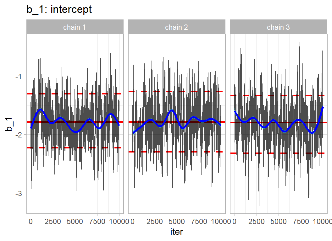
trace_plot(simDF, b_2) +
  labs(title="b_2: number missing squared")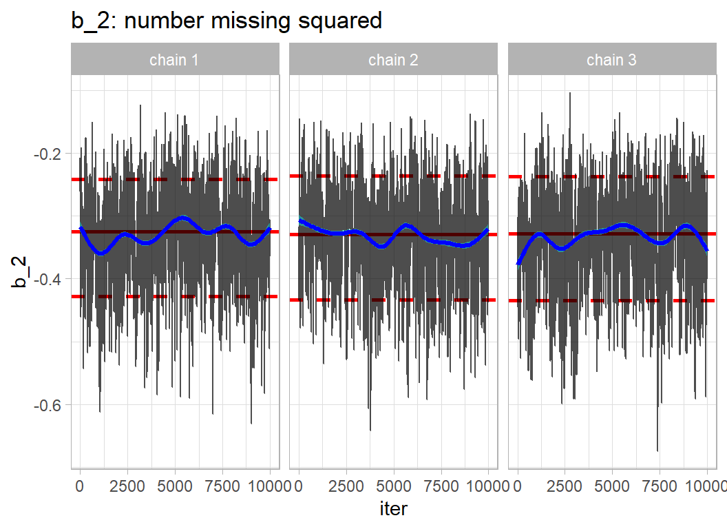
trace_plot(simDF, b_3) +
  labs(title="b_3: APPROACH")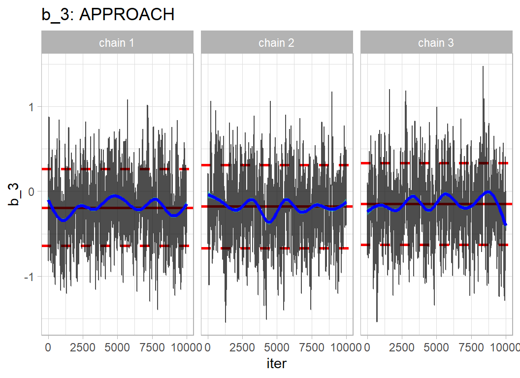
trace_plot(simDF, b_10) +
  labs(title="b_10: TAXI")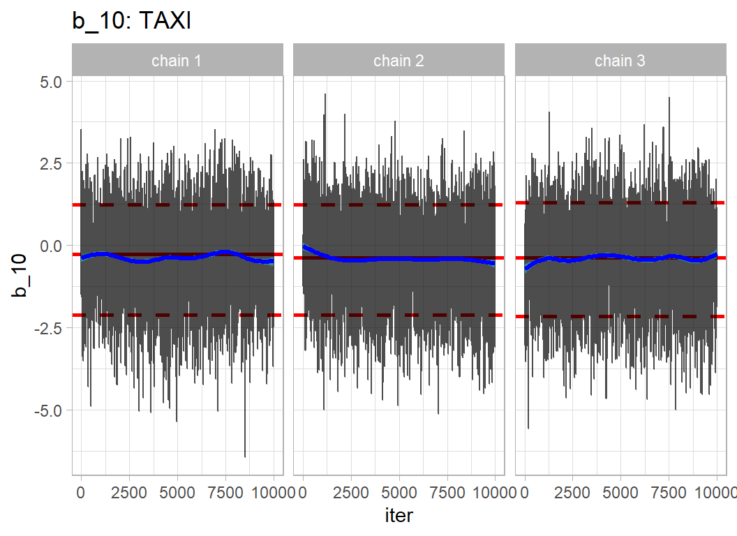
The high autocorrelation is expected given the high correlation between parameters. The chains have converged, but the long run length was essential to provide sufficient accuracy.
Below I create a table of summary statistics for comparing the Bayesian and Likelihood analyses.
# --- LIKELIHOOD ANALYSIS ---------------------------------------
sampleDF %>%
  mutate( nmiss  = nmiss - 1.5,
          nmiss2 = nmiss * nmiss ) %>%
  glm( damaged ~ nmiss2 + flight_phase,
       family = "binomial", data = .) %>%
  tidy() %>%
  select(estimate, std.error) -> glmDF


# --- Bayesian results ------------------------------------------
library(coda)

codaSims <- mcmc(simDF %>% select(-chain, -iter))

summary(codaSims)[[1]] %>%
  as_tibble( rownames="term") %>%
  select( -`Naive SE`) %>%
  rename( MCMC_Error = `Time-series SE`) %>%
  bind_cols(glmDF) %>% print()
## # A tibble: 10 × 6
## term Mean SD MCMC_Error estimate std.error
## <chr> <dbl> <dbl> <dbl> <dbl> <dbl>
## 1 b_1 -1.79 0.381 0.0184 -1.72 0.423
## 2 b_2 -0.332 0.0762 0.00244 -0.311 0.0746
## 3 b_3 -0.171 0.369 0.0144 -0.270 0.399
## 4 b_4 -0.517 0.477 0.0129 -0.594 0.515
## 5 b_5 -0.462 0.482 0.0141 -0.535 0.516
## 6 b_6 0.810 0.391 0.0134 0.745 0.422
## 7 b_7 0.942 0.550 0.0179 0.977 0.588
## 8 b_8 0.735 0.824 0.0140 1.03 0.858
## 9 b_9 -0.672 1.22 0.0153 -13.3 725.
## 10 b_10 -0.393 1.32 0.0160 -13.1 1029.The MCMC_Error shows that the algorithm estimates the posterior means to within about 0.03 (i.e. twice the MCMC error).
The likelihood and Bayesian analyses are in broad agreement both in terms of the posterior mean and the posterior standard deviation. The Bayesian estimates for b_9 and b_10 are more sensible and I would prefer to use them for prediction rather than the values from the likelihood analysis.
Model Comparison
As well as the number of missing values and the phase of the flight, the size of the aircraft and the size of the bird or animal are also important, but the importance of the quantity of the wildlife is less clear-cut. Here is a summary of the unadjusted species_quantity effect.
# --- Effect of number of animals/birds --------------------------
sampleDF %>%
  group_by( species_quantity) %>%
  summarise( n = n(),
             damaged = sum(damaged),
             pct = 100*damaged / n,
             logit = log( pct/(100 - pct)))
## # A tibble: 4 × 5
## species_quantity n damaged pct logit
## <fct> <int> <dbl> <dbl> <dbl>
## 1 1 1209 63 5.21 -2.90
## 2 2-10 122 11 9.02 -2.31
## 3 (Missing) 35 3 8.57 -2.37
## 4 11-100 9 1 11.1 -2.08Broadly, as you might expect, the more wildlife, the more likely that the aircraft is damaged. The counts are not large, especially when we remember that model will adjust for other predictors.
A traditional analysis, would judge the contribution of species_quantity by an analysis of deviance table
# --- LIKELIHOOD ANALYSIS ---------------------------------------
sampleDF %>%
  mutate( nmiss  = nmiss - 1.5,
          nmiss2 = nmiss * nmiss ) %>%
  glm( damaged ~ nmiss2 + flight_phase + aircraft_mass + size +
          species_quantity,
       family = "binomial", data = .) %>%
  anova()
## Analysis of Deviance Table
##
## Model: binomial, link: logit
##
## Response: damaged
##
## Terms added sequentially (first to last)
##
##
## Df Deviance Resid. Df Resid. Dev
## NULL 1374 599.13
## nmiss2 1 59.547 1373 539.58
## flight_phase 8 20.999 1365 518.58
## aircraft_mass 5 23.125 1360 495.46
## size 5 86.003 1355 409.46
## species_quantity 3 6.017 1352 403.44Assuming that the model assumptions hold (I have not checked them yet) then the deviance can be judged by a chi-squared test.
pchisq(6.017, 3, lower=FALSE)## [1] 0.1107861So the test for addition of species_quantity has a p-value of 0.11, suggesting that the evidence for adding species_quantity is pretty weak.
Bayesian Model Comparison
The traditional analysis compares the base model with the expanded model in terms of the difference in their deviances. In contrast, a Bayesian analysis either compares the models in terms of either their posterior probability, or their Bayes Factor.
Posterior probability is perhaps the purest measure, but it requires the analyst to give a prior on the probability that the “correct” model includes species_quantity.
In contrast, the Bayes Factor calculates the change between the prior odds of two models and their posterior odds; that is to say, it measures the impact of the data on the model choice. On the ratio of odds scale, that change is independent of what we originally thought about the inclusion of species_quantity.
I will look at both Bayesian approaches in one analysis.
I need a prior for the probability based method. In my opinion, there is an 80% chance that species quantity is predictive of damage after adjusting for the other factors. I tend to the view that the lack of significance in the likelihood analysis is down to the sparsity of the data.
My prior odds for including species_quantity is therefore 0.8/(1-0.8) = 4.
Model Probability
I need to create an MCMC algorithm that is free to switch between the two models (i.e. with and without species_quantity) and I do this by including an indicator variable in my model code.
The nimble run follows much the same pattern as before. First, I set up the data in a list().
# ==============================================================
# NIMBLE ANALYSIS
#

# --- Place data in a list -------------------------------------
Y <- sampleDF$damaged

sampleDF %>%
  mutate( nmiss  = nmiss - 1.5,
          nmiss2 = nmiss * nmiss ) %>%
  { model.matrix( ~ nmiss2 + flight_phase + aircraft_mass + size +
          species_quantity, data=.) } -> X

myData <- list(X=X, Y=Y)

saveRDS( myData, file.path(home, "nimble/data02.rds"))
In my model code, I include the indicator, zSQ, (z for Species Quantity) which is zero when species_quantity is omitted from the model and one when that predictor is included. In each iteration, a Metropolis-Hastings algorithm will decide whether zSQ should be 0 or 1. This algorithm will require values for the coefficients of species_quantity even when previously zSQ was 0. The values that are used for the coefficients of the unused predictor are arbitrary and will not alter the solution. However, they can have a big impact on the speed of convergence. Choose poorly and the algorithm will be very slow to switch from a model without species_quantity (zSQ=0) to one with species_quantity (zSQ=1). A sensible choice would be to use values close to the mean coefficient in a model that includes species_quantity. I use a likelihood analysis to help guide that choice.
# --- LIKELIHOOD ANALYSIS ---------------------------------------
sampleDF %>%
  mutate( nmiss  = nmiss - 1.5,
          nmiss2 = nmiss * nmiss ) %>%
  glm( damaged ~ nmiss2 + flight_phase + aircraft_mass + size +
          species_quantity,
       family = "binomial", data = .) %>%
  tidy() %>%
  slice(21:23)
## # A tibble: 3 × 5
## term estimate std.error statistic p.value
## <chr> <dbl> <dbl> <dbl> <dbl>
## 1 species_quantity2-10 0.358 0.425 0.842 0.400
## 2 species_quantity(Missing) 1.72 0.876 1.96 0.0495
## 3 species_quantity11-100 2.25 1.17 1.92 0.0548The distribution that is used to create regression coefficients for terms not in the model is called a pseudo-prior. In the code below, my pseudo-priors are based on this likelihood analysis, remembering that the choice only needs to be sensible; there is no correct choice.
# --- Model in BUGS style --------------------------------------
library(nimble)

nimbleCode( {
  # Prior on the probability of including species_quantity
   zSQ ~ dbern(0.8)

  # zSQ (0/1) indicates whether species quantity is included
  # z[] are indicators for the 23 columns of X
   for( j in 1:20) {
      z[j] <- 1
   }
   for(j in 21:23) {
     z[j] <- zSQ
   }
  # the likelihood
   for( i in 1:1375) {
     for(j in 1:23 ) {
       a[i,j] <- z[j] * b[j] * X[i,j]
     }
     logit(p[i]) <- sum(a[i, 1:23])
     Y[i] ~ dbern(p[i])
   }
  # Priors on the coefficients b[1:23]
  # intercept
   b[1] ~ dnorm(-4.0, sd = 2)
  # number missing
   b[2] ~ dnorm(-0.5, sd = 0.25)
  # log odds ratios
   for( j in 3:20 ) {
     b[j] ~ dnorm(0.0, sd = 1.5)
   }
  # First level of species quantity
  # prior zSQ=1 N(0, 1.5), pseudo prior zSQ=0 N(0.4, 0.25)
   m21 <- (1 - zSQ)*0.4
   s21 <- (1 - zSQ)/4 + zSQ * 1.5
   b[21] ~ dnorm( m21, sd = s21)
  # Second level of species quantity
  # prior zSQ=1 N(0, 1.5), pseudo prior zSQ=0 N(2, 0.5)
   m22 <- (1 - zSQ)*2
   s22 <- (1 - zSQ)/2 + zSQ * 1.5
   b[22] ~ dnorm( m22, sd = s22)
  # third level of species quantity
  # prior zSQ=1 N(0, 1.5), pseudo prior zSQ=0 N(2, 0.5)
   m23 <- (1 - zSQ)*2
   s23 <- (1 - zSQ)/2 + zSQ * 1.5
   b[23] ~ dnorm( m23, sd = s23)
} ) -> myCode

saveRDS( myCode, file.path(home, "nimble/model02.rds"))
The run proceeds as before.
# --- tibble to control the analysis --------------------------
set.seed(1582)
tibble(
  model   = file.path(home, "nimble/model02.rds"),
  data    = file.path(home, "nimble/data02.rds"),
  niter   = rep(20000, 3),
  nburnin = rep(10000, 3),
  thin    = rep(1, 3),
  seed   = c(3456, 2398, 3477),
  inits   = list(
  list( b = rnorm(23, c(-4, -0.5, rep(0, 21)), sd=0.1), zSQ=1),
  list( b = rnorm(23, c(-4, -0.5, rep(0, 21)), sd=0.1), zSQ=1),
  list( b = rnorm(23, c(-4, -0.5, rep(0, 21)), sd=0.1), zSQ=1) ),
  sims    = paste(
    file.path(home, "data/dataStore/sims02_"), 1:3,".rds", sep="")
) %>%
  print() -> designDF
## # A tibble: 3 × 8
## model data niter nburnin thin seed inits sims
## <chr> <chr> <dbl> <dbl> <dbl> <dbl> <list> <chr>
## 1 C:/Projects/kaggle/Sliced/… C:/P… 20000 10000 1 3456 <named list> C:/P…
## 2 C:/Projects/kaggle/Sliced/… C:/P… 20000 10000 1 2398 <named list> C:/P…
## 3 C:/Projects/kaggle/Sliced/… C:/P… 20000 10000 1 3477 <named list> C:/P…# --- Run three chains in parallel --------------------------
library(furrr)
# --- run three independent R sessions --------------
plan(multisession, workers=3)
# --- run the chains in parallel --------------------
designDF %>%
future_pwalk(run_nimble) %>%
system.time()
# --- switch back to sequential processing ----------
plan(sequential)This run took 244 seconds. Here are some trace plots based on the analysis.
# --- Read the simulations into a tibble ------------
simDF <- bayes_to_df(designDF$sims)

# --- Some trace plots ------------------------------
trace_plot(simDF, b_1) +
  labs(title="b_1: intercept")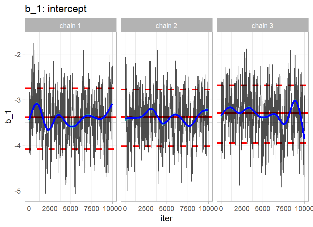
trace_plot(simDF, b_2) +
  labs(title="b_2: number missing squared")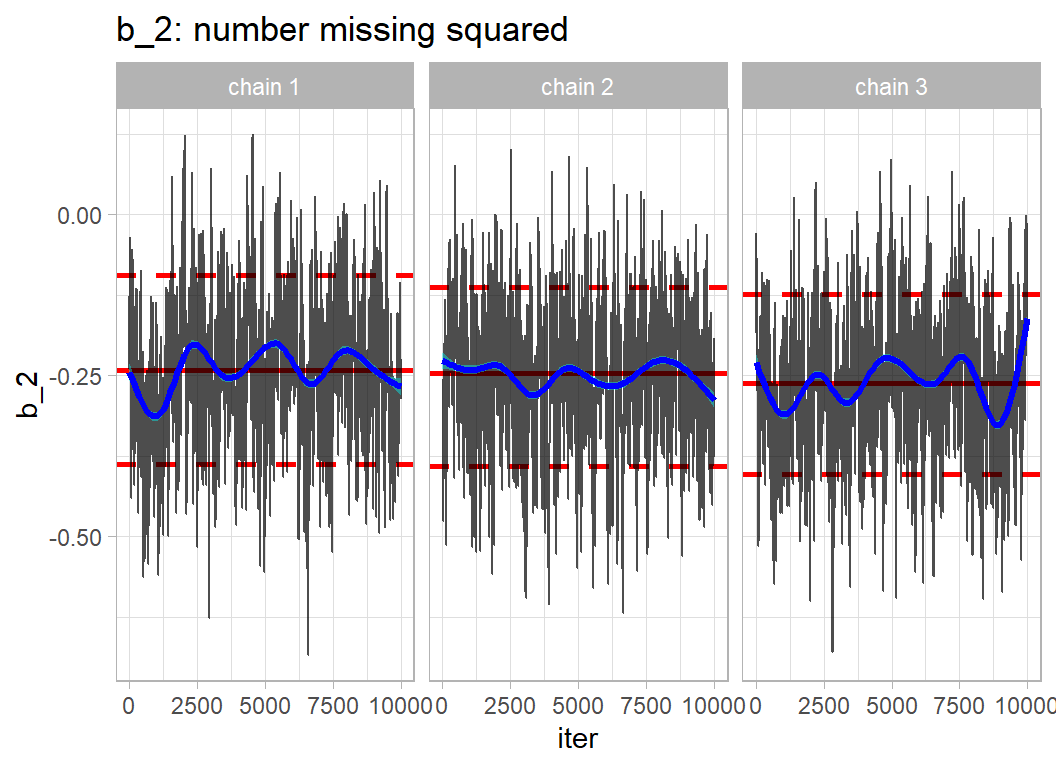
trace_plot(simDF %>% filter(zSQ==1), b_21) +
  labs(title="b_21: Quantity 2-10, drawn from the posterior")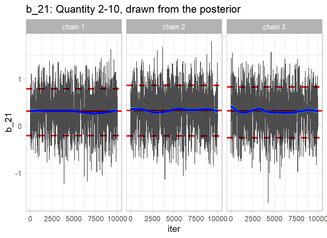
trace_plot(simDF %>% filter(zSQ==0), b_21) +
  labs(title="b_21: Quantity 2-10, drawn from the pseudo prior")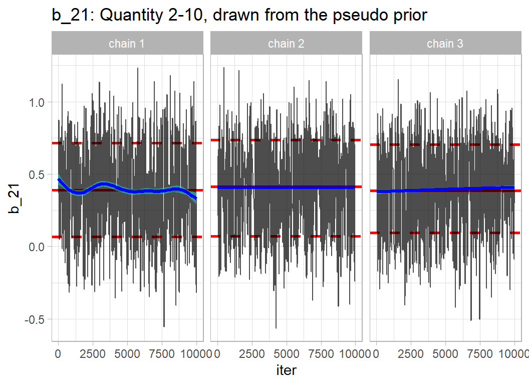
trace_plot(simDF %>% filter(zSQ==1), b_23) +
  labs(title="b_23: Quantity 11-100, drawn from the posterior")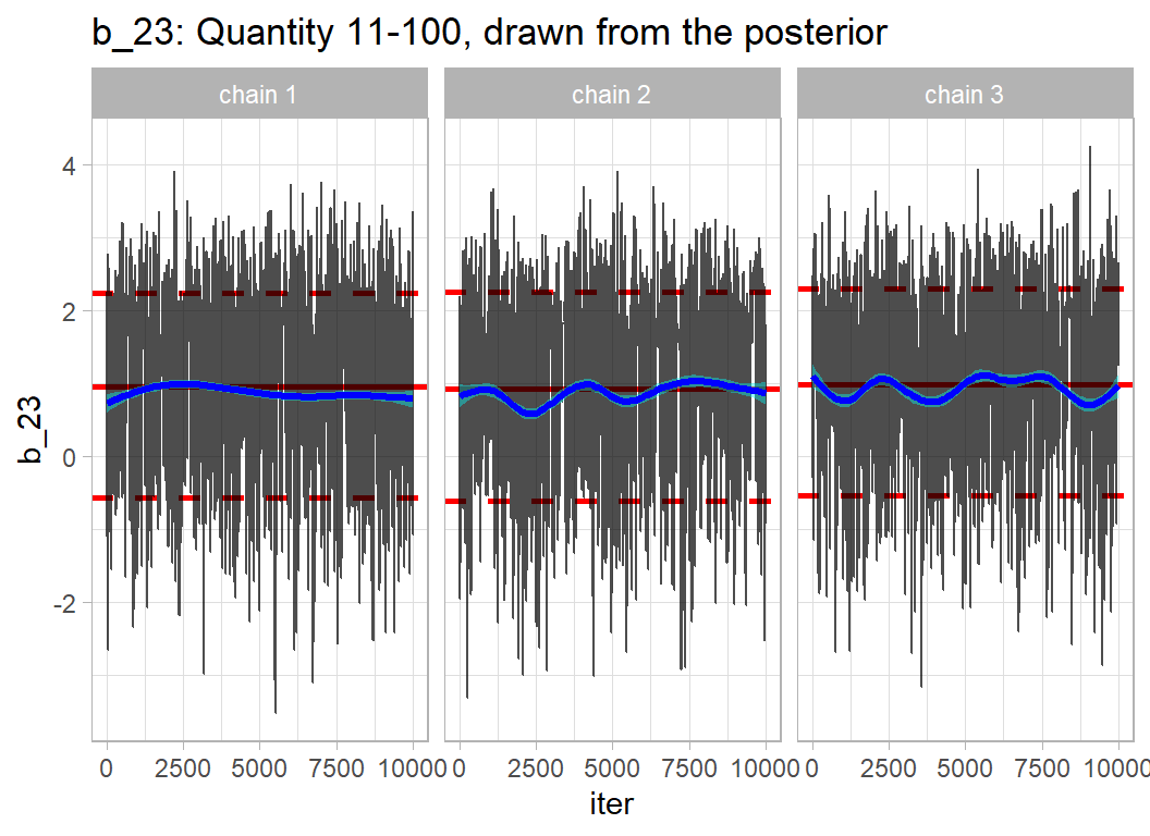
trace_plot(simDF %>% filter(zSQ==0), b_23) +
  labs(title="b_23: Quantity 11-100, drawn from the pseudo prior")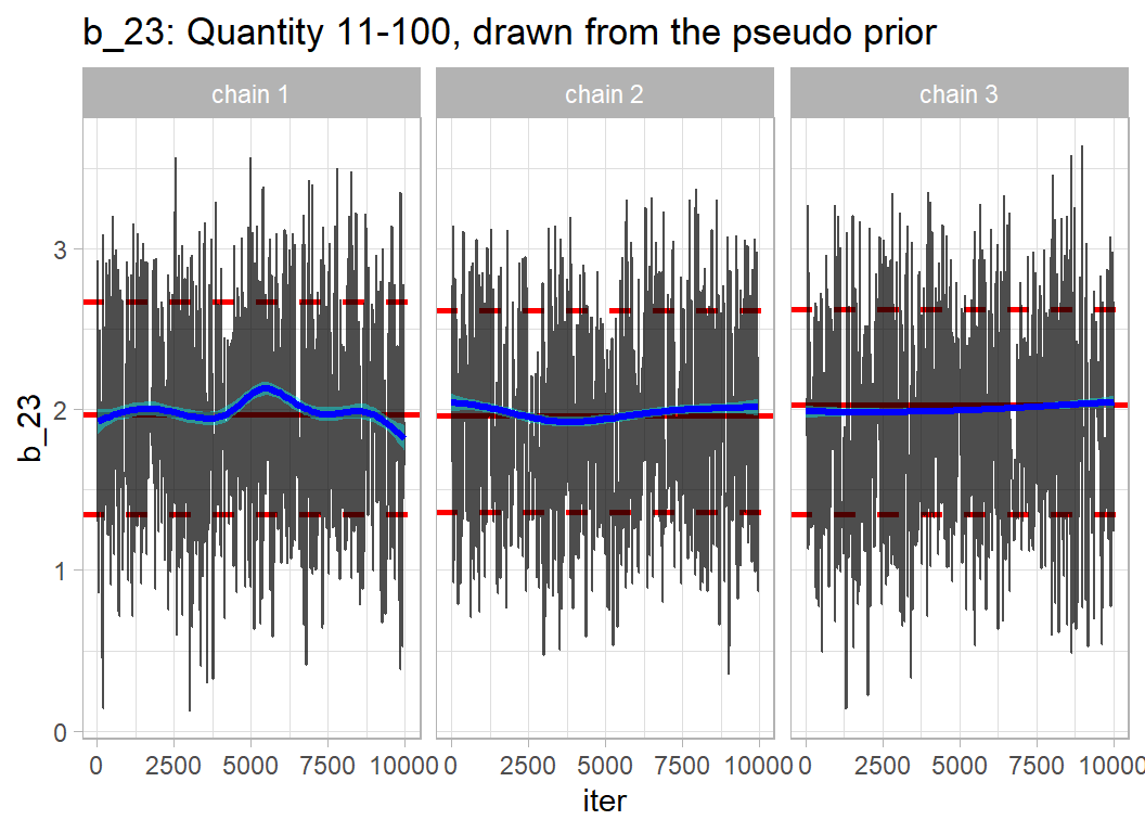
trace_plot(simDF, zSQ) +
  labs(title="zSQ: Whether to include species_quantity")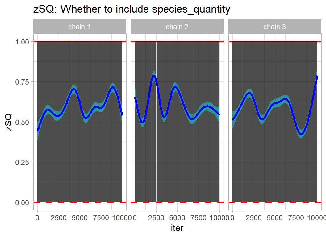
table(simDF$zSQ)##
## 0 1
## 12186 17814So after adjusting for the data, the posterior probability that the model includes species_quantity is 17814/30000=0.59 and the posterior odds is 0.59/(1-0.59)=1.43
The data have caused me to adjust my odds by a factor of 1.43/4 = 0.36, this is the Bayes Factor. The data move me away from including species_quantity, from 80% sure to 59% sure, a drop by a factor of 0.36 in the odds.
The data have not had a big influence, because there is not much data. If you had started believing that the including species_quantity was 50:50, i.e a probability of 0.5 and an odds of 1, the data would have reduced your odds by the same Bayes Factor, so your new odds would have been 0.36, equivalent to a posterior probability of 0.26.
What we learn from this analysis
In the past, I have run this type of analysis in OpenBUGS with reasonable results and I was interested to see whether or not nimble is a practical alternative. The answer seems to be a qualified yes. The default in nimble for non-conjugate parameters is to use a random walk Metropolis-Hastings algorithm that is automatically tuned prior during the burn-in. The algorithm is quick, but my experience suggests that very long run lengths are needed for all but the most trivial models.
nimble is an ambitious project that offers a wide range of other samplers, but the user is left to search for the best combination of samplers without much guidance from the package. I am a fan of leaving the analyst in control, but even I would like a more intelligent choice of default behaviour. At present, nimble does not include an HMC algorithm, which is a shame as that algorithm works without much tuning from the analyst and would serve as a better default.
My approach to Bayesian analysis differs from that of the majority of statisticians in that I believe in the use of informative priors. Most people are happier with vague priors that leave the data to dictate the model fit. This example has illustrated some of the advantages of my preferred approach.
Informative priors produce more sensible estimates when the data are sparse. In the first model, we saw how the likelihood analysis, which is equivalent to a bayesian model with a very vague prior, gave log odds ratio estimates of -13, equivalent to an odds ratio of around 2x10⁻⁶. Since damage is a reasonably uncommon outcome the odds ratio approximates a ratio of probabilities, so the model would have us believe that a missing flight phase is 2 million times more risky than one in the TAXI category.
It is usually the case that MCMC algorithms converge faster when the priors are informative. An MCMC algorithm will try to cover the posterior. In the case of the TAXI category the likelihood analysis suggests a standard error of around 1000, this gives us a good indication of the size of the posterior standard deviation. So the algorithm will try to cover parameter values in the range -2000 to +2000. Not only are these values ridiculous, but they run the risk of crashing the run due to numerical overflow or overflow.
Vague priors are sometimes not quite as vague as was intended. This would almost certainly not be a problem for this example, but with more complex models a supposedly vague prior on one parameter can have an unanticipated impact on other parameters, perhaps limiting their range.
Informative priors allow the analyst to use extra knowledge with the potential for better predictions. Birdstrikes are more common during periods of migration, some aircraft incorporate extra safety features to protect against birdstrikes and some airports do more than others to keep wildlife away. If you know such things, it is sensible to make use of that information.
The final aspect that was touched upon in this post is the contrast between p-values and Bayes Factors for model comparison. The p-value of 0.11 associated adding species_quantity to the model is hard to interpret. Is it non-significant due to the poor predictive performance of that measure, or is it due to low sample size? With large datasets that are more the norm in machine learning, the opposite behaviour is often observed. Small p-values arise from adding predictors that make no material contribution to overall performance and machine learning models often become unnecessarily complex.
The interpretation of a Bayes Factor of 0.36 is more direct, especially when it is converted to a model probability. I started with a prior probability of 0.8 that species_quantity should be included, equivalent to odds ratio of 4. The data gave a BF of 0.36, so combining my prior with the data reduced the odds ratio to 4x0.36=1.43, which translates into a posterior probability of 0.59. One can see that the data do not help with the decision and we have a metric on an easily understood probability scale.