Bayesian Sliced 3: Superstore profits
Summary:
Background: In episode 3 of the 2021 series of Sliced, the competitors were given two hours in which to analyse a set of data on superstore sales. The aim was to predict the profit on each sale in the test set.
My approach: I start with the model used in my non-Bayesian analysis of these data, which transformed the profit to the profit that would have been obtained had there not been a discount. I use this example to illustrate analysis with stan and so I start by using stan to fit an equivalent Bayesian model. Noting that the variance is not constant across sub-categories of items, I extend the Bayesian model and then used a Bayes Factor to compare the original and the modified Bayesian models.
Result: My first Bayesian model gives almost the same results to a linear model fitted with lm(). The modified model gives similar posterior means, but very different posterior standard deviations. The Bayes Factor greatly favours the modified analysis.
Conclusion: The modified model makes similar predictions to a basic linear model, but it conveys much more information, in particular, it identifies those predictions that are made with high confidence and those that are more uncertain.
Introduction
The third of the Sliced tasks is to predict the profits on items sold by a unnamed superstore and as usual the evaluation metric is RMSE. The data can be downloaded from https://www.kaggle.com/c/sliced-s01e03-DcSXes.
I analysed these profit data in an earlier post called Spliced Episode 3: Siperstore profits. I cleaned the data, explored the individual predictors and used a linear regression model for prediction. The problem illustrates the importance of using known structure when modelling data. In this particular case, I use the data on discounts to convert all profits to what they would have been without a discount. I then developed a predictive model for the undiscounted profit.
This is the third of a series of posts in which I re-analyse the Sliced data using Bayesian methods. I will not repeat the data cleaning and visualisation and so this post needs to be read in conjunction with my earlier post.
Reading the data
I will pick up the previous analysis at the point where I read the clean data. The transformations between sales and undiscounted sales (baseSales) and between profit and undiscounted profit (baseProfit) are explained in the earlier post.
# --- setup: libraries & options ------------------------
library(tidyverse)

theme_set( theme_light())

# --- set home directories ------------------------------
oldHome <- "C:/Projects/sliced/s01-e03"
home    <- "C:/Projects/sliced/Bayes-s01-e03"

# --- read downloaded data -----------------------------
readRDS( file.path(oldHome, "data/rData/train.rds") ) %>%
  mutate( baseSales  = sales / (1 - discount),
          baseProfit = profit + sales * discount / (1 - discount) ) -> trainDF
Models
Linear Model
I will start with the model structure used in my original post. It was created with the code
library(broom)

# --- base model: coefficients -----------------------------
trainDF %>%
  filter( baseProfit > 0.5 ) %>%
  { lm( log10(baseProfit) ~  - 1 + sub_category,
              offset=log10(baseSales),
              data=.) } %>%
  tidy() %>%
  select( -statistic) %>%
  mutate(term = str_replace(term, "sub_category", "")) %>%
  print() -> modDF
## # A tibble: 17 × 4
## term estimate std.error p.value
## <chr> <dbl> <dbl> <dbl>
## 1 Accessories -0.590 0.00862 0
## 2 Appliances -0.536 0.0109 0
## 3 Art -0.508 0.00844 0
## 4 Binders -0.323 0.00621 0
## 5 Bookcases -0.747 0.0154 0
## 6 Chairs -0.691 0.00961 0
## 7 Copiers -0.359 0.0295 7.73e- 34
## 8 Envelopes -0.323 0.0147 1.18e-103
## 9 Fasteners -0.418 0.0176 2.76e-120
## 10 Furnishings -0.520 0.00784 0
## 11 Labels -0.324 0.0124 1.18e-142
## 12 Machines -0.434 0.0229 2.79e- 78
## 13 Paper -0.324 0.00632 0
## 14 Phones -0.614 0.00805 0
## 15 Storage -0.894 0.00846 0
## 16 Supplies -0.774 0.0181 0
## 17 Tables -0.728 0.0133 0The model consists of a series of 45o lines one for each sub_category of product. The intercepts are log10 of the proportion of the sales price that goes in profit.
trainDF %>%
  filter( baseProfit > 0.5 ) %>%
  { lm( log10(baseProfit) ~  sub_category,
              offset=log10(baseSales),
              data=.) } %>%
  augment() %>%
  arrange( sub_category, `(offset)`) %>%
  ggplot( aes(x=`(offset)`, y=.fitted, colour=sub_category)) +
  geom_line() +
  labs( x= "log10(baseSales)", y="log10(baseProfit)",
        title = "Predicted profit for a given undiscounted sales price")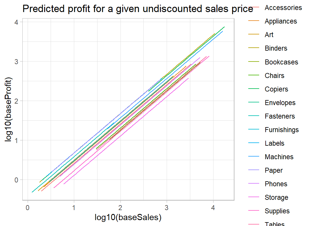
The main limitation of the this model is that it assumes that it is possible to predict profits in every sub-category with the same accuracy. We know from my previous analysis that this is not true. Some sub-categories are quite homogeneous, but other include items that produce very different percentage profit. This effect can be seen in the plot below.
# --- profit and sales for 3 categories of item -------------
trainDF %>%
  mutate( baseSales  = sales / (1 - discount),
          baseProfit = profit + sales * discount / (1 - discount) ) %>%
  mutate( discount = factor(discount)) %>%
  filter( baseProfit > 0.5 ) %>%
  filter( sub_category %in% c("Tables", "Phones", "Binders") ) %>%
  ggplot( aes(x=log10(baseSales), y=log10(baseProfit)) ) +
  geom_point() +
  geom_abline( slope=1, intercept=0) +
  facet_wrap( ~ sub_category) +
  labs( title="Undiscounted profit and  sales price on a log scale")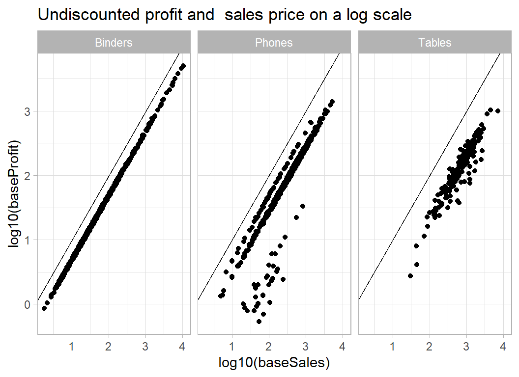
The variation about the trend line varies considerably with sub-category.
Linear Model in Stan
Despite the limitations of the linear model with constant variance, I start with its equivalent in stan and then I’ll improve the Bayesian model.
Here is the model code for the equivalent to the linear model.
data {
  int N;               // number of data points i.e. 7087
  int M;               // number of sub_categories of product 17
  vector[N] Y;         // the response log10(baseProfit)
  vector[N] sales;     // log10(baseSales)
  int cat[N];          // sub-category 1-17
}
parameters {
  vector[M] a;                // coefficients
  real<lower=0> sigma;        // sd about regression line
  real<lower=0> tau;          // sd of sub_category avg profit
}
transformed parameters {
  vector[N] Yhat;             // fitted values
  Yhat = sales + a[cat];
}
model {
  Y ~ normal(Yhat, sigma);    // regression model
  a ~ normal(0, tau);         // prior on coefficients
  sigma ~ cauchy(0, 1);       // vague prior on sd of model
  tau ~ cauchy(0, 1);         // vague prior on sd of sub_cat
}
I saved this model code in a text file called profit_mod1.stan within a folder called stan.
The data are prepared and stored in a list.
# --- transform the data ----------------------------------
trainDF %>%
  filter( baseProfit > 0.5 ) %>%
  mutate( Y = log10(baseProfit),
          S = log10(baseSales),
          C = as.numeric( factor(sub_category))) -> tempDF

# --- Save in a list() ------------------------------------
stanData <- list( N=7087, M=17,
                   Y     = tempDF$Y,
                   sales = tempDF$S,
                   cat   = tempDF$C )
stan runs 3 chains in parallel in 90 seconds on my desktop. The computation took about 5 seconds and the rest of the time was taken with compilation and saving the results.
# --- fit model using stan --------------------------------
library(rstan)

stan(file   = 'stan/profit_mod1.stan',
     data   = stanData,
     chains = 3,
     cores  = 3,
     iter   = 2000,
     warmup = 1000,
     pars   = c("a", "sigma", "tau"),
     seed   = 3982) %>%
  saveRDS( file.path(home, "data/dataStore/profit_mod1.rds")) %>%
  system.time()
The results are saved in stan format, but can be extracted by my stan_to_df() function as described in the methods post on Bayesian Software.
library(MyPackage)

readRDS( file.path(home, "data/dataStore/profit_mod1.rds")) %>%
  stan_to_df() %>%
  print() -> sim1DF
## # A tibble: 6,000 × 22
## chain iter a_1 a_2 a_3 a_4 a_5 a_6 a_7 a_8 a_9 a_10 a_11
## <fct> <int> <dbl> <dbl> <dbl> <dbl> <dbl> <dbl> <dbl> <dbl> <dbl> <dbl> <dbl>
## 1 1 1 1.84 1.54 0.357 1.55 0.678 0.650 -1.42 1.45 0.171 1.77 -1.92
## 2 1 2 1.84 1.54 0.357 1.55 0.678 0.650 -1.42 1.45 0.171 1.77 -1.92
## 3 1 3 1.84 1.54 0.357 1.55 0.678 0.650 -1.42 1.45 0.171 1.77 -1.92
## 4 1 4 1.84 1.54 0.357 1.55 0.678 0.650 -1.42 1.45 0.171 1.77 -1.92
## 5 1 5 1.84 1.54 0.357 1.55 0.678 0.650 -1.42 1.45 0.171 1.77 -1.92
## 6 1 6 1.83 1.54 0.354 1.53 0.679 0.643 -1.42 1.45 0.162 1.75 -1.91
## 7 1 7 1.82 1.53 0.347 1.51 0.683 0.634 -1.42 1.45 0.161 1.73 -1.91
## 8 1 8 1.78 1.52 0.315 1.46 0.683 0.610 -1.44 1.43 0.168 1.68 -1.88
## 9 1 9 1.77 1.53 0.313 1.45 0.689 0.607 -1.44 1.43 0.160 1.68 -1.88
## 10 1 10 1.72 1.51 0.270 1.37 0.677 0.590 -1.41 1.42 0.172 1.60 -1.88
## # … with 5,990 more rows, and 9 more variables: a_12 <dbl>, a_13 <dbl>,
## # a_14 <dbl>, a_15 <dbl>, a_16 <dbl>, a_17 <dbl>, sigma <dbl>, tau <dbl>,
## # lp__ <dbl>The results file includes the warmup in which the algorithm is tuned, so this portion needs to be discarded. You only need to look at it when something goes wrong.
The likelihood analysis with lm() estimated the intercept to be -0.59 with a standard error of 0.009, very close to the Bayesian posterior.
# --- trace plot of the first coefficient -------------------
sim1DF %>%
  filter( iter > 1000 ) %>%
  trace_plot(a_1, "Accessories")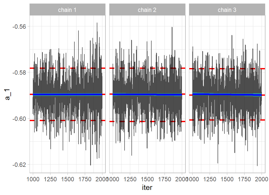
Convergence is very good and the results mirror those of the model fitted by lm().
## # A tibble: 17 × 5
##    term          lmCf    lmSe bay1Mn  bay1Sd
##    <chr>        <dbl>   <dbl>  <dbl>   <dbl>
##  1 Accessories -0.590 0.00862 -0.590 0.00889
##  2 Appliances  -0.536 0.0109  -0.536 0.0105
##  3 Art         -0.508 0.00844 -0.508 0.00810
##  4 Binders     -0.323 0.00621 -0.323 0.00628
##  5 Bookcases   -0.747 0.0154  -0.746 0.0155
##  6 Chairs      -0.691 0.00961 -0.691 0.00923
##  7 Copiers     -0.359 0.0295  -0.358 0.0305
##  8 Envelopes   -0.323 0.0147  -0.323 0.0147
##  9 Fasteners   -0.418 0.0176  -0.418 0.0177
## 10 Furnishings -0.520 0.00784 -0.520 0.00780
## 11 Labels      -0.324 0.0124  -0.323 0.0127
## 12 Machines    -0.434 0.0229  -0.433 0.0223
## 13 Paper       -0.324 0.00632 -0.323 0.00634
## 14 Phones      -0.614 0.00805 -0.614 0.00825
## 15 Storage     -0.894 0.00846 -0.894 0.00852
## 16 Supplies    -0.774 0.0181  -0.774 0.0179
## 17 Tables      -0.728 0.0133  -0.728 0.0133
Improved Bayesian Model
The modified model has a different standard deviation for each sub-category of product. The log(sd) of each sub-category is assumed to be drawn from a normal distribution with unknown precision.
data {
  int N;           // number of data points i.e. 7087
  int M;           // number of sub_categories of product 17
  vector[N] Y;     // the response log10(baseProfit)
  vector[N] sales; // log10(baseSales)
  int cat[N];      // sub-category 1-17
}
parameters {
  vector[M] a;            // coefficients
  vector[M] logsigma;     // log of sd about regression line
  real<lower=0> tau;      // sd of sub_category avg profit
  real<lower=0> psi;      // sd of sub_category logsigma
}
transformed parameters {
  vector[M] sigma;
  sigma = exp(logsigma);
}
model {
  Y ~ normal(sales + a[cat], sigma[cat]);    // regression model
  a ~ normal(-0.65, tau);        // prior on coefficients
  logsigma ~ normal(-1.5, psi);  // vague prior on sd of model
  tau ~ cauchy(0, 1);            // vague prior on sd of sub_cat
  psi ~ cauchy(0, 1);            // vague prior on sd of logsigma
}
The prior on a[] is centred on -0.65 and as we are modelling the log10 undiscounted profit, this is equivalent to a profit of around 20%-25%. Looking at the linear model coefficients, this profit is probably a little low, but it is not unreasonable. The figure must, of course, be chosen without reference to these data. It is my guess at what profit stores might make.
The distribution of log(sd) is centred on -1.5, equivalent to a standard deviation of about 0.2. So, if the coefficient for a sub-category were -0.65, I would be allowing items within that sub-category to vary between about -0.25 and -1.05, equivalent to profits between 9% and and 56%.
I could have chosen to replace my guesses, -0.65 and -1.5, which unknown parameters, placed a prior on those parameters and then allowed the data to have a say in their values. I have not tried it, but my feeling is that it would make very little difference.
Fitting precedes in the same way.
# --- fit model using stan ------------------------------------------
stan(file = 'stan/profit_mod2.stan',
     data = stanData,
     chains = 3,
     cores  = 3,
     iter   = 2000,
     warmup = 1000,
     pars   = c("a", "sigma", "tau", "psi")) %>%
  saveRDS( file.path(home, "data/dataStore/profit_mod2.rds")) %>%
  system.time()
The model takes a similar time to compile, but much longer to run, about 100 seconds as opposed to 5 seconds.
The posterior means for the modified model are very similar to those of the original model, but the posterior standard deviations are very different, reflecting the greater uncertainty about the profit in some sub-categories compared to others.
## # A tibble: 17 × 7
##    term          lmCf    lmSe bay1Mn  bay1Sd bay2Mn   bay2Sd
##    <chr>        <dbl>   <dbl>  <dbl>   <dbl>  <dbl>    <dbl>
##  1 Accessories -0.590 0.00862 -0.590 0.00889 -0.590 0.0100
##  2 Appliances  -0.536 0.0109  -0.536 0.0105  -0.536 0.00298
##  3 Art         -0.508 0.00844 -0.508 0.00810 -0.508 0.00333
##  4 Binders     -0.323 0.00621 -0.323 0.00628 -0.323 0.000432
##  5 Bookcases   -0.747 0.0154  -0.746 0.0155  -0.746 0.0137
##  6 Chairs      -0.691 0.00961 -0.691 0.00923 -0.691 0.00894
##  7 Copiers     -0.359 0.0295  -0.358 0.0305  -0.360 0.0104
##  8 Envelopes   -0.323 0.0147  -0.323 0.0147  -0.323 0.00101
##  9 Fasteners   -0.418 0.0176  -0.418 0.0177  -0.421 0.0211
## 10 Furnishings -0.520 0.00784 -0.520 0.00780 -0.520 0.00776
## 11 Labels      -0.324 0.0124  -0.323 0.0127  -0.324 0.000667
## 12 Machines    -0.434 0.0229  -0.433 0.0223  -0.434 0.0129
## 13 Paper       -0.324 0.00632 -0.323 0.00634 -0.324 0.000411
## 14 Phones      -0.614 0.00805 -0.614 0.00825 -0.614 0.0118
## 15 Storage     -0.894 0.00846 -0.894 0.00852 -0.892 0.0192
## 16 Supplies    -0.774 0.0181  -0.774 0.0179  -0.771 0.0361
## 17 Tables      -0.728 0.0133  -0.728 0.0133  -0.728 0.00940
Bayes Factor
Now that we have two competing Bayesian models, the obvious question is whether the more complex model fits any better.
When comparing two models, say \(M_1\) and \(M_2\), for a set of data, \(y\), Bayes theorem tells us that \[ \frac{p(M_1 \ | \ y)}{p(M_2 \ | \ y)} = \frac{p(y \ | \ M_1) \ \ p(M_1)}{p(y \ | \ M_2) \ \ p(M_2)} \] In words the ratio of the posterior probability of model \(M_1\) to model \(M_2\) is equal to the ratio of the marginal likelihoods times the ratio of the prior probabilities. The ratio of the marginal likelihoods is known as the Bayes Factor (BF) and it captures the way that the data cause us to modify our prior beliefs about the two models. A BF of 1 would tells us that the data have had no impact on our beliefs, while a large BF says that the data have moved us towards \(M_1\) and a small BF says that we have been moved towards \(M_2\).
In my Bayesian post on the wildlife strike data (episode 2) I calculated the Bayes Factor for comparing two models using pseudo priors and an algorithm that was free to move between the two models. In that way, I was able to calculate the ratio of the posterior probabilities and since I fixed the prior probabilities, I was able to deduce the BF.
By way of contrast, I will calculate the marginal likelihoods of my models directly and then find the Bayes Factor as the their ratio. Calculation of the marginal likelihoods is not trivial. You will notice that the parameters of the models do not appear in the updating formula; this is because they are integrated out of the marginal likelihoods.
\[ p(y \ | \ M_1) = \int p(y \ | \ \theta, M_1) \ \ p(\theta \ | \ M_1) \ \ d\theta \]
I will drop the conditioning on \(M_1\) and introduce an arbitrary proposal distribution \(g(\theta)\).
\[ p(y) = \frac{\int p(y \ | \ \theta) \ \ p(\theta) \ g(\theta) \ \ d\theta}{\int \frac{p(y \ | \ \theta) \ \ p(\theta)}{p(y)} \ g(\theta) \ \ d\theta} \]
which reduces to \[ p(y) = \frac{\int p(y \ | \ \theta) \ \ p(\theta) \ g(\theta) \ \ d\theta}{\int \ g(\theta) \ \ p(\theta \ | \ y) \ d\theta} \]
The top integral can be approximated using a sample of values of \(\theta\) drawn from the proposal distribution and the lower integral can be approximated using a sample of values from the posterior. The MCMC algorithm has provided a sample from the posterior and the proposal distribution is deliberately chosen so that it is easy to sample from.
\[ p(y) = \frac{E_g \left\{ p(y \ | \ \theta) \ \ p(\theta) \right\} } { E_p \left\{ g(\theta) \right\} } \]
So far we have employed classic importance sampling. The method works, but its accuracy is highly dependent on choosing a proposal that closely resembles the posterior. To improve the accuracy, we could add a second function \(h(\theta)\) to the top and bottom. \(h(\theta)\) is called a bridge function, because it is chosen to bridge the gap between the posterior and the proposal.
\[ p(y) = \frac{E_g \left\{ p(y \ | \ \theta) \ \ p(\theta) \ h(\theta) \right\} } { E_p \left\{ g(\theta) \ h(\theta) \right\} } \]
Our remaining problem is to choose \(h(\theta)\), since it bridges the gap between the proposal and the posterior, the optimal choice will depend on both distributions. The proposal distribution is not a problem, because it is chosen by us and so is known exactly. The posterior is a problem, because it must be known exactly, which means that we need to know the normalising constant \(p(y)\). This is just the marginal likelihood that we set out to find. We have entered a loop and the solution requires us to iterate. Guess \(p(y)\), find the bridge function \(h(\theta)\), re-calculate \(p(y)\), refine the bridge function and so on until convergence. Fortunately, this process has been automated in an R package called bridgesampling.
When we calculate a likelihood ratio for comparing two alternative sets of parameters from the same distribution, the constants in the formula for the density can be dropped as they cancel. These constants are also dropped when MCMC algorithms sample from the posterior. However, when the marginal likelihood is required, it is vital that these constants are retained. To do this in Stan, the model code needs to be written in a different way. The log posterior (target) is accumulated in a series of calls to the log probability density functions (lpdf) of the distributions.
Here is the re-structured code for model 1.
data {
  int N;           // number of data points i.e. 7087
  int M;           // number of sub_categories of product 17
  vector[N] Y;     // the response log10(baseProfit)
  vector[N] sales; // log10(baseSales)
  int cat[N];      // sub-category 1-17
}
parameters {
  vector[M] a;            // coefficients
  real<lower=0> sigma;    // sd about regression line
  real<lower=0> tau;      // sd of sub_category avg profit
}
transformed parameters {
  vector[N] Yhat;          // fitted values
  Yhat = sales + a[cat];
}
model {
  target += normal_lpdf(Y | Yhat, sigma );
  target += normal_lpdf(a | 0, tau);
  target += cauchy_lpdf(sigma | 0, 1);
  target += cauchy_lpdf(tau | 0, 1);
}
I placed this code in a file called profit_mod1bf.stan and rather than use the stan() function, I sampled from the posterior in two stages. stan_model() compiles the code and sampling() runs the HMC sampler, in this case with default values for number and length of chains, etc.
# --- compile the model code ------------------------------
stanmodelH1 <- stan_model(file = 'stan/profit_mod1bf.stan',
                          model_name="stanmodel1")

# --- sample from the posterior ---------------------------
stanfitH1 <- sampling(stanmodelH1, data = stanData)
The bridgesampling package can now be used to evaluate the log of the marginal likelihood.
library(bridgesampling)

# --- use bridge sampling to approximate the marginal likelihood ---
mod1Bridge <- bridge_sampler(stanfitH1, silent = TRUE)
The package approximates the integral and gives an indication of the accuracy of its approximation. In this case, the log marginal likelihood is about 1203 as calculated after 5 iterations of the bridge sampling and is accurate to within about 1%. If you need more accuracy, run stan’s sampler for longer.
# --- print the marginal likelihood -------------------------------
print(mod1Bridge)
## Bridge sampling estimate of the log marginal likelihood: 1203.436
## Estimate obtained in 5 iteration(s) via method "normal".# --- print the percentage error of the approximation -------------
error_measures(mod1Bridge)$percentage## [1] "1%"Next, I run the equivalent calculations for the second model, which has different standard deviations for each category of product.
# --- print the marginal likelihood -------------------------------
print(mod2Bridge)
## Bridge sampling estimate of the log marginal likelihood: 8323.309
## Estimate obtained in 6 iteration(s) via method "normal".# --- print the percentage error in the approximation -------------
error_measures(mod2Bridge)$percentage## [1] "1%"The log marginal likelihood is 8323. So the Bayes Factor in favour of model 2 is exp(8323-1203), which is off-the-scale huge. There is a slightly unnecessary function that performs this calculation
# --- find the Bayes Factor ---------------------------------------
bf(mod2Bridge, mod1Bridge)
## Estimated Bayes factor in favor of mod2Bridge over mod1Bridge: InfThe evidence in favour of model 2 is Inf, i.e. overwhelming.
What this example shows:
The model with difference variances for each class of product provides a massively better fit to the data, as we already knew from the plots made for the original analysis of these data. Yet, the point predictions under the two models are almost identical, so a Bayesian statistician sees model 2 as being much better, while a data scientist concludes that the two models are almost equivalent. The difference, of course, is that the two are interested in different things. The Bayesian is concerned with the predictive distribution, not just the point prediction. For this problem, we can make separate predictions for accessories and office furniture, but we know that the accuracy of those predictions will vary. For some product types, we expect our prediction to be highly accurate, because the profit is similar for everything within that category, while for more variable categories the prediction will be much less reliable. The Bayesian cares about this difference, while machine learning with its reliance on a loss function, does not.