Bayesian Sliced 4: Rain Tomorrow
Summary:
Background: In episode 4 of the 2021 series of Sliced, the competitors were given two hours to analyse a set of data on rainy days in Australia. The aim was to use today’s weather data to predict whether or not it will rain tomorrow.
My approach: In this post, I use a series of hierarchical models, where the location within Australia is one level and day within the location is the other. I fit the models by both likelihood and Bayesian methods. I finish by running a Bayesian analysis across different imputed datasets in order to adjust for the uncertainty introduced by missing values.
Result: Bayesian models fitted with stan give very similar estimates to models fitted by maximum likelihood with glmer, although the Bayesian models are more robust and are less likely to run into convergence issues.
Conclusion: Hierarchical models are a natural option for weather data on days within locations. However, this dataset is large with many days of weather data for each city, so it is possible to create a good within city model without the need to learn from the experience of other cities. For big data problems, the gains from hierarchical modelling are limited.
Introduction
The fourth of the Sliced tasks is to predict whether or not it will rain tomorrow based on weather records for 49 different locations in Australia. The data can be downloaded from https://www.kaggle.com/c/sliced-s01e04-knyna9..
In my original post, I analysed the 49 locations separately and used the appropriate model to make my predictions. I noted at the time that a hierarchical model would have been preferable, but I resisted the temptation to fit such a model, because I knew that it would be computationally demanding and I had already spent a lot of time on the data cleaning and the imputation of missing values.
In this post, I investigate the use of hierarchical models for these data. I start by fitting the models by maximum likelihood; this requires numerical integration and the algorithm can be numerically unstable when the number of parameters is large, or when the random effects have small variances. Then, I fit equivalent Bayesian hierarchical models in stan. I use the brms package to prepare the stan code.
I adjust the final model for the uncertainty due to the missing values by repeating the Bayesian analysis on each of five imputed datasets.
Reading the data
In the original post, I cleaned the data and, because of the number of missing values, I used the mice package to impute five sets of complete data. I pick up the analysis by reading the first of those multiple imputations.
# --- setup: libraries & options ------------------------
library(tidyverse)
library(mice)

theme_set( theme_light())

# --- set home directory -------------------------------
oldHome <- "C:/Projects/sliced/s01-e04"
home    <- "C:/Projects/sliced/Bayes-s01-e04"

# --- read results from mice ---------------------------
imp2 <- readRDS(file.path(oldHome, "data/rData/imp2.rds"))

# --- extract 1st set of imputed training data ---------
complete(imp2, action=1) %>%
  slice( 1:34191 ) %>%
  as_tibble() -> trainDF

# --- select 15000 observations for estimation ----------
set.seed(8231)
split <- sample(1:34191, size=15000, replace=FALSE)

# --- extract training data and scale ------------------
trainDF %>%
  slice(split) %>%
    mutate( across( contains("3pm"), scale),
            wind_gust_speed = scale(wind_gust_speed)) -> estimateDF
I deliberately make the estimation set relatively small (n = 15,000) in order than the model development is speeded up. Hierarchical models are slow to fit, whatever algorithm you use.
Convergence of both likelihood and Bayesian analyses is improved when the explanatory variables are measured over similar ranges, so I scale the continuous variables that I plan to use in my models.
The need for a hierarchical structure
In my previous post, I analysed each location separately, for example, here is a typical model fitted to the data from Perth in Western Australia. The offset logitBayes is the logit of the probability that it will rain on any given day during that month in that location as estimated from the training data. It acts as a baseline when estimating the logit of the probability of rain_tomorrow.
library(broom)
# --- glm for Perth -------------------------------------------
estimateDF %>%
  filter( location == "Perth") %>%
  glm( rain_tomorrow ~ rain_today + humidity3pm +
           temp3pm + pressure3pm + wind_speed3pm,
           family="binomial", offset=logitBayes, data=.) %>%
  tidy()
## # A tibble: 6 × 5
## term estimate std.error statistic p.value
## <chr> <dbl> <dbl> <dbl> <dbl>
## 1 (Intercept) -0.249 0.287 -0.869 0.385
## 2 rain_today1 0.309 0.430 0.720 0.472
## 3 humidity3pm 1.44 0.350 4.11 0.0000403
## 4 temp3pm -0.277 0.377 -0.734 0.463
## 5 pressure3pm -1.87 0.315 -5.94 0.00000000281
## 6 wind_speed3pm -0.120 0.339 -0.356 0.722Not surprisingly, high humidity is associated with an increased chance of rain the following day. Analysing all 49 locations (not shown) indicates that the sizes of these associations do vary from location to location, but the broad pattern is the same everywhere.
It makes sense to think of an average humidity effect for all Australia with individual cities varying randomly about that average. These variations will follow a zero-centred distribution and by building that distribution into the analysis, the estimate of the humidity effect for Perth will be influenced by the humidity effects in other locations, hopefully making Perth’s estimate more accurate and more numerically stable.
In locations where the humidity effect is either unusually large or unusually small, the random effect will move that estimate towards the centre of the distribution, that is, towards Australia’s average effect size. This phenomenon, usually called shrinkage, ought to protect against extreme predictions based on little data.
Likelihood analysis with glmer()
The hierarchical structure leads us to a so-called mixed model; mixed because if includes both a fixed effect and a random effect. The fixed effect is the average across all of Australia and the random effect is the variation between locations.
The function lmer() from the package lmer fits mixed models when the response is normally distributed. The calculation of the likelihood requires integration over the random effects, which are modelled as being zero-centred normal distributions. The joint normality means that the likelihood can be integrated analytically, greatly simplifying the algorithm.
When the response is not normally distributed, mixed models are fitted with the glmer() function, also from the lmer package; it is an extension of the glm() function. Once again, the random effects are modelled as being zero-centred normal distributions, but now the integral is intractable and it needs to be approximated numerically.
The glmer algorithm maximises a likelihood that, at each stage, is evaluated by numerical integration. The algorithm is slow and can be unstable. Stability is improved by adding more points to the numerical integration, but then the algorithm becomes even slower.
As well as the fixed effects, such as the average humidity effect for all of Australia, the algorithm estimates the variances of the zero-centred random effects. In situations where there is not much variation between locations, such variances will be small and the algorithm has to search for a solution that lies on, or close to, the edge of the parameter space. This is notoriously difficult to do in a numerically stable way.
A model with a random intercept
The first model is a logistic regression for the binary response rain_tomorrow (Yes=1, No=0) with three predictors and an offset.
Without a hierarchical structure this is just a generalized linear model that can be fitted by glm().
# --- Model 1: fitted by glm ----------------------------------
glm(rain_tomorrow ~ 1 + rain_today + humidity3pm + pressure3pm,
              family=binomial(link=logit),
              offset = logitBayes,
              data = estimateDF) %>%
  { tidy(.) %>%
      print()
    glance(.) %>%
      print()}
## # A tibble: 4 × 5
## term estimate std.error statistic p.value
## <chr> <dbl> <dbl> <dbl> <dbl>
## 1 (Intercept) -0.655 0.0329 -19.9 4.21e- 88
## 2 rain_today1 0.514 0.0518 9.93 3.06e- 23
## 3 humidity3pm 1.15 0.0313 36.6 8.05e-294
## 4 pressure3pm -0.707 0.0251 -28.2 2.96e-175
## # A tibble: 1 × 8
## null.deviance df.null logLik AIC BIC deviance df.residual nobs
## <dbl> <int> <dbl> <dbl> <dbl> <dbl> <int> <int>
## 1 14978. 14999 -5923. 11853. 11884. 11845. 14996 15000The intercept measures the deviation from the offset when the other predictors are zero, i.e. no rain_today, national average humidity and pressure. This intercept can be allowed to vary by location by adding a random effect.
# --- Model 1: mixed model fitted by glmer --------------------
library(lme4)

glmer(rain_tomorrow ~ 1 + rain_today + humidity3pm + pressure3pm +
        ( 1 | location),
              family=binomial(link="logit"),
              offset = logitBayes,
              data = estimateDF) %>%
  summary()
## Generalized linear mixed model fit by maximum likelihood (Laplace
## Approximation) [glmerMod]
## Family: binomial ( logit )
## Formula: rain_tomorrow ~ rain_today + humidity3pm + pressure3pm + (1 |
## location)
## Data: .
## Offset: logitBayes
##
## AIC BIC logLik deviance df.resid
## 11521.9 11560.0 -5756.0 11511.9 14995
##
## Scaled residuals:
## Min 1Q Median 3Q Max
## -5.7835 -0.4234 -0.2173 -0.0704 11.0584
##
## Random effects:
## Groups Name Variance Std.Dev.
## location (Intercept) 0.3652 0.6043
## Number of obs: 15000, groups: location, 49
##
## Fixed effects:
## Estimate Std. Error z value Pr(>|z|)
## (Intercept) -0.62565 0.09278 -6.743 1.55e-11 ***
## rain_today1 0.44598 0.05264 8.473 < 2e-16 ***
## humidity3pm 1.36971 0.03486 39.287 < 2e-16 ***
## pressure3pm -0.76493 0.02659 -28.770 < 2e-16 ***
## ---
## Signif. codes: 0 '***' 0.001 '**' 0.01 '*' 0.05 '.' 0.1 ' ' 1
##
## Correlation of Fixed Effects:
## (Intr) rn_td1 hmdty3
## rain_today1 -0.159
## humidity3pm -0.116 -0.223
## pressure3pm 0.069 0.060 -0.190The fixed effects are similar to those of the glm() model, but the extra random term, (1 | location), allows the intercepts to vary by location. Over Australia as a whole, the intercept is 0.626. However, this intercept is not uniform across the country; the intercepts over the 49 locations have an estimated variance of 0.365.
A model with random coefficients
The previous model assumed that the impacts of the predictors, rain_today, humidity and pressure, are the same everywhere. So, although the intercept, which represents the chance of rain tomorrow when there is no rain today, is allowed to vary with location, the difference between no rain today and some rain today is assumed to be the same everywhere.
The next model allows the coefficients of the predictors to vary as well as the intercept.
# --- Model 2: mixed model fitted by glmer --------------------

glmer(rain_tomorrow ~ 1 + rain_today + humidity3pm + pressure3pm +
        ( 1  + rain_today + humidity3pm + pressure3pm | location),
              family=binomial(link="logit"),
              offset = logitBayes,
              data = estimateDF) %>%
  summary()
## Generalized linear mixed model fit by maximum likelihood (Laplace
## Approximation) [glmerMod]
## Family: binomial ( logit )
## Formula: rain_tomorrow ~ rain_today + humidity3pm + pressure3pm + (1 +
## rain_today + humidity3pm + pressure3pm | location)
## Data: .
## Offset: logitBayes
##
## AIC BIC logLik deviance df.resid
## 11145.5 11252.1 -5558.7 11117.5 14986
##
## Scaled residuals:
## Min 1Q Median 3Q Max
## -8.4369 -0.4166 -0.2120 -0.0601 12.1173
##
## Random effects:
## Groups Name Variance Std.Dev. Corr
## location (Intercept) 0.3544 0.5953
## rain_today1 0.1532 0.3913 -0.89
## humidity3pm 0.1080 0.3287 -0.01 0.02
## pressure3pm 0.3302 0.5746 -0.57 0.67 0.55
## Number of obs: 15000, groups: location, 49
##
## Fixed effects:
## Estimate Std. Error z value Pr(>|z|)
## (Intercept) -0.55164 0.09335 -5.909 3.43e-09 ***
## rain_today1 0.32331 0.08068 4.007 6.14e-05 ***
## humidity3pm 1.47979 0.06101 24.255 < 2e-16 ***
## pressure3pm -0.75999 0.08776 -8.660 < 2e-16 ***
## ---
## Signif. codes: 0 '***' 0.001 '**' 0.01 '*' 0.05 '.' 0.1 ' ' 1
##
## Correlation of Fixed Effects:
## (Intr) rn_td1 hmdty3
## rain_today1 -0.685
## humidity3pm -0.069 -0.116
## pressure3pm -0.462 0.459 0.359The average impact of each of these predictors is significant and the effect sizes vary with location. The variances of the random effects indicate that there is wide variation in the intercepts and pressure coefficients, but less variation in the coefficient of humidity and rain today.
The default for glmer is to assume that all of the random effects are correlated and the results table gives the estimates of those correlations. For instance, the intercept and rain_today have an estimated correlation of -0.89. So, in places where the intercept is high, the effect of rain today tends to be smaller.
To illustrate the range of models that glmer() can fit, I try a slight variation on this model. I remove the random effect on rain today that is, I assume that rain today has the same effect everywhere. Then, I assume that the random effect on the intercept and random effects on the other predictors are independent.
# --- MODEL 3: simplified glmer model ------------------------
estimateDF %>%
  glmer(rain_tomorrow ~ 1 + rain_today + humidity3pm + pressure3pm +
              (1 | location) +
              (0 + humidity3pm + pressure3pm | location),
              offset = logitBayes,
              family=binomial(link=logit),
              data = .) %>%
  summary()
## Generalized linear mixed model fit by maximum likelihood (Laplace
## Approximation) [glmerMod]
## Family: binomial ( logit )
## Formula: rain_tomorrow ~ rain_today + humidity3pm + pressure3pm + (1 |
## location) + (0 + humidity3pm + pressure3pm | location)
## Data: .
## Offset: logitBayes
##
## AIC BIC logLik deviance df.resid
## 11179.7 11240.6 -5581.9 11163.7 14992
##
## Scaled residuals:
## Min 1Q Median 3Q Max
## -7.9636 -0.4187 -0.2130 -0.0636 11.3659
##
## Random effects:
## Groups Name Variance Std.Dev. Corr
## location (Intercept) 0.2663 0.5160
## location.1 humidity3pm 0.1138 0.3373
## pressure3pm 0.3318 0.5760 0.59
## Number of obs: 15000, groups: location, 49
##
## Fixed effects:
## Estimate Std. Error z value Pr(>|z|)
## (Intercept) -0.58504 0.08303 -7.047 1.83e-12 ***
## rain_today1 0.42408 0.05404 7.848 4.23e-15 ***
## humidity3pm 1.45286 0.06145 23.644 < 2e-16 ***
## pressure3pm -0.74178 0.08811 -8.419 < 2e-16 ***
## ---
## Signif. codes: 0 '***' 0.001 '**' 0.01 '*' 0.05 '.' 0.1 ' ' 1
##
## Correlation of Fixed Effects:
## (Intr) rn_td1 hmdty3
## rain_today1 -0.170
## humidity3pm -0.077 -0.143
## pressure3pm 0.042 0.023 0.402Notice that the fixed effects sizes are very similar to those in the model with the more general correlation structure. Removing the correlation makes the computation quicker and more stable, but the model may be a little unrealistic.
Bayesian mixed models with stan
The main differences between likelihood and Bayesian mixed models are the priors and fitting algorithm. The priors, especially those on the variances, should improve convergence and, as the Bayesian algorithm uses simulation, it does not require numerical integration. The combined effect is that the Bayesian algorithm should be more stable. However, a Bayesian analysis needs to simulate parameters for every location and the Bayesian algorithm will be slower.
I have a choice, I could either write my own stan code, or I could use brms or stanarm. These packages contain functions that write the stan code for you. I have opted to use brms.
I start with the brms equivalent of model 2.
# --- Model 2 fitted with stan via brms -------------------
library(brms)

estimateDF %>%
  brm(rain_tomorrow ~ 1 + rain_today + humidity3pm + pressure3pm +
              offset(logitBayes) +
              (1 + rain_today + humidity3pm + pressure3pm | location),
              family=bernoulli(link=logit),
              data = .,
              prior = c(prior(normal(0, 1), class = Intercept),
              prior(normal(0, 1), class = b),
              prior(normal(0, 1), class = sd)),
      iter = 2000, warmup = 1000, thin = 1,
      chains = 4, cores = 4, seed = 3491) %>%
  summary()
## Family: bernoulli
## Links: mu = logit
## Formula: rain_tomorrow ~ 1 + rain_today + humidity3pm + pressure3pm + offset(logitBayes) + (1 + rain_today + humidity3pm + pressure3pm | location)
## Data: . (Number of observations: 15000)
## Draws: 4 chains, each with iter = 2000; warmup = 1000; thin = 1;
## total post-warmup draws = 4000
##
## Group-Level Effects:
## ~location (Number of levels: 49)
## Estimate Est.Error l-95% CI u-95% CI Rhat Bulk_ESS
## sd(Intercept) 0.60 0.08 0.46 0.77 1.00 1171
## sd(rain_today1) 0.39 0.08 0.24 0.56 1.00 1517
## sd(humidity3pm) 0.35 0.07 0.23 0.48 1.00 1045
## sd(pressure3pm) 0.59 0.07 0.47 0.74 1.00 1563
## cor(Intercept,rain_today1) -0.78 0.12 -0.95 -0.47 1.00 1958
## cor(Intercept,humidity3pm) 0.01 0.18 -0.35 0.37 1.00 1546
## cor(rain_today1,humidity3pm) -0.01 0.23 -0.45 0.43 1.00 541
## cor(Intercept,pressure3pm) -0.49 0.13 -0.71 -0.22 1.00 1408
## cor(rain_today1,pressure3pm) 0.57 0.16 0.23 0.84 1.01 551
## cor(humidity3pm,pressure3pm) 0.49 0.16 0.15 0.77 1.00 1570
## Tail_ESS
## sd(Intercept) 1821
## sd(rain_today1) 2169
## sd(humidity3pm) 2318
## sd(pressure3pm) 2162
## cor(Intercept,rain_today1) 2419
## cor(Intercept,humidity3pm) 2110
## cor(rain_today1,humidity3pm) 1466
## cor(Intercept,pressure3pm) 1939
## cor(rain_today1,pressure3pm) 1389
## cor(humidity3pm,pressure3pm) 2168
##
## Population-Level Effects:
## Estimate Est.Error l-95% CI u-95% CI Rhat Bulk_ESS Tail_ESS
## Intercept -0.55 0.09 -0.72 -0.36 1.00 781 1472
## rain_today1 0.32 0.08 0.16 0.49 1.00 1521 1955
## humidity3pm 1.47 0.06 1.36 1.60 1.00 2312 3072
## pressure3pm -0.76 0.09 -0.95 -0.58 1.00 1296 1947
##
## Draws were sampled using sampling(NUTS). For each parameter, Bulk_ESS
## and Tail_ESS are effective sample size measures, and Rhat is the potential
## scale reduction factor on split chains (at convergence, Rhat = 1).The fixed effect estimates are almost identical to those given by glmer. brm() reports standard deviations rather than variances, but once again they are almost identical to those of glmer, although the correlation is a little smaller, perhaps because of the independent priors. In this case glmer and stan are effectively equivalent.
A more complex model
In my previous post on these data, I got reasonable results with a location-specific model based on rain_today, humidity, pressure, temperature and wind speed in the afternoon and the wind gust speed. Here is the glmer version of the equivalent mixed model.
# --- model 4: more complex mixed model -------------------------------
estimateDF %>%
  glmer(rain_tomorrow ~ 1 + rain_today +
                humidity3pm + pressure3pm + temp3pm +
                wind_speed3pm + wind_gust_speed +
                (1 + rain_today +
                humidity3pm + pressure3pm + temp3pm +
                wind_speed3pm + wind_gust_speed | location),
                offset = logitBayes,
                family=binomial(link=logit),
                data = .) %>%
  summary()
## Generalized linear mixed model fit by maximum likelihood (Laplace
## Approximation) [glmerMod]
## Family: binomial ( logit )
## Formula: rain_tomorrow ~ 1 + rain_today + humidity3pm + pressure3pm +
## temp3pm + wind_speed3pm + wind_gust_speed + (1 + rain_today +
## humidity3pm + pressure3pm + temp3pm + wind_speed3pm + wind_gust_speed |
## location)
## Data: .
## Offset: logitBayes
##
## AIC BIC logLik deviance df.resid
## 10638.7 10905.2 -5284.3 10568.7 14965
##
## Scaled residuals:
## Min 1Q Median 3Q Max
## -13.1222 -0.3861 -0.2001 -0.0543 14.2249
##
## Random effects:
## Groups Name Variance Std.Dev. Corr
## location (Intercept) 0.36010 0.6001
## rain_today1 0.11847 0.3442 -0.88
## humidity3pm 0.15070 0.3882 0.49 -0.35
## pressure3pm 0.21952 0.4685 -0.23 0.55 0.40
## temp3pm 0.19312 0.4395 0.55 -0.59 0.54 -0.15
## wind_speed3pm 0.05653 0.2378 -0.23 0.09 -0.20 -0.27 0.04
## wind_gust_speed 0.03664 0.1914 0.64 -0.35 0.38 0.16 0.25 -0.78
## Number of obs: 15000, groups: location, 49
##
## Fixed effects:
## Estimate Std. Error z value Pr(>|z|)
## (Intercept) -0.48124 0.09635 -4.995 5.89e-07 ***
## rain_today1 0.18161 0.07867 2.309 0.021 *
## humidity3pm 1.69105 0.07384 22.902 < 2e-16 ***
## pressure3pm -0.52628 0.07738 -6.801 1.04e-11 ***
## temp3pm 0.10208 0.08016 1.273 0.203
## wind_speed3pm -0.34072 0.05375 -6.339 2.32e-10 ***
## wind_gust_speed 0.80301 0.04990 16.092 < 2e-16 ***
## ---
## Signif. codes: 0 '***' 0.001 '**' 0.01 '*' 0.05 '.' 0.1 ' ' 1
##
## Correlation of Fixed Effects:
## (Intr) rn_td1 hmdty3 prssr3 tmp3pm wnd_s3
## rain_today1 -0.615
## humidity3pm 0.288 -0.265
## pressure3pm -0.153 0.344 0.313
## temp3pm 0.379 -0.235 0.508 0.040
## wind_spd3pm -0.108 0.051 -0.075 -0.130 0.047
## wnd_gst_spd 0.308 -0.178 0.253 0.165 0.142 -0.678
## optimizer (Nelder_Mead) convergence code: 4 (failure to converge in 10000 evaluations)
## Model failed to converge with max|grad| = 0.0218223 (tol = 0.002, component 1)
## failure to converge in 10000 evaluationsNotice that the algorithm failed to converge
Although glmer did not converge, the solution is probably roughly OK. It suggests that temperature and rain_today are of minor importance. Wind speeds are important, but the coefficients don’t vary much from place to place.
Here is the Bayesian version of the same mixed model.
# --- model 4 fitted by stan -------------------------------------
estimateDF %>%
  brm(rain_tomorrow ~ 1 + rain_today +
                humidity3pm + pressure3pm + temp3pm +
                wind_speed3pm + wind_gust_speed +
                offset(logitBayes) +
                (1 + rain_today +
                humidity3pm + pressure3pm + temp3pm +
                wind_speed3pm + wind_gust_speed | location),
              family=bernoulli(link=logit),
              data = .,
              prior = c(prior(normal(0, 1), class = Intercept),
              prior(normal(0, 1), class = b),
              prior(cauchy(0, 1), class = sd)),
      iter = 2000, warmup = 1000, thin = 1,
      chains = 4, cores = 4, seed = 3491) %>%
  summary()
## Family: bernoulli
## Links: mu = logit
## Formula: rain_tomorrow ~ 1 + rain_today + humidity3pm + pressure3pm + temp3pm + wind_speed3pm + wind_gust_speed + offset(logitBayes) + (1 + rain_today + humidity3pm + pressure3pm + temp3pm + wind_speed3pm + wind_gust_speed | location)
## Data: . (Number of observations: 15000)
## Draws: 4 chains, each with iter = 2000; warmup = 1000; thin = 1;
## total post-warmup draws = 4000
##
## Group-Level Effects:
## ~location (Number of levels: 49)
## Estimate Est.Error l-95% CI u-95% CI Rhat
## sd(Intercept) 0.60 0.07 0.47 0.76 1.00
## sd(rain_today1) 0.33 0.08 0.18 0.49 1.00
## sd(humidity3pm) 0.39 0.07 0.26 0.53 1.00
## sd(pressure3pm) 0.49 0.07 0.37 0.63 1.00
## sd(temp3pm) 0.46 0.07 0.33 0.61 1.00
## sd(wind_speed3pm) 0.17 0.07 0.03 0.31 1.00
## sd(wind_gust_speed) 0.13 0.06 0.02 0.26 1.00
## cor(Intercept,rain_today1) -0.66 0.15 -0.89 -0.30 1.00
## cor(Intercept,humidity3pm) 0.34 0.17 -0.01 0.65 1.00
## cor(rain_today1,humidity3pm) -0.19 0.22 -0.59 0.27 1.00
## cor(Intercept,pressure3pm) -0.19 0.17 -0.49 0.15 1.00
## cor(rain_today1,pressure3pm) 0.46 0.18 0.07 0.77 1.00
## cor(humidity3pm,pressure3pm) 0.34 0.17 -0.02 0.65 1.00
## cor(Intercept,temp3pm) 0.40 0.16 0.05 0.68 1.00
## cor(rain_today1,temp3pm) -0.39 0.20 -0.75 0.03 1.00
## cor(humidity3pm,temp3pm) 0.37 0.18 -0.01 0.67 1.00
## cor(pressure3pm,temp3pm) -0.15 0.18 -0.50 0.21 1.00
## cor(Intercept,wind_speed3pm) -0.07 0.24 -0.53 0.42 1.00
## cor(rain_today1,wind_speed3pm) -0.03 0.27 -0.54 0.51 1.00
## cor(humidity3pm,wind_speed3pm) -0.10 0.26 -0.59 0.42 1.00
## cor(pressure3pm,wind_speed3pm) -0.22 0.23 -0.65 0.27 1.00
## cor(temp3pm,wind_speed3pm) 0.12 0.24 -0.37 0.59 1.00
## cor(Intercept,wind_gust_speed) 0.42 0.25 -0.17 0.82 1.00
## cor(rain_today1,wind_gust_speed) -0.18 0.29 -0.70 0.42 1.00
## cor(humidity3pm,wind_gust_speed) 0.20 0.29 -0.41 0.71 1.00
## cor(pressure3pm,wind_gust_speed) 0.05 0.28 -0.54 0.55 1.00
## cor(temp3pm,wind_gust_speed) 0.17 0.27 -0.39 0.65 1.00
## cor(wind_speed3pm,wind_gust_speed) -0.29 0.33 -0.80 0.44 1.00
## Bulk_ESS Tail_ESS
## sd(Intercept) 1626 2560
## sd(rain_today1) 2410 2898
## sd(humidity3pm) 2171 2671
## sd(pressure3pm) 2670 3254
## sd(temp3pm) 2439 2951
## sd(wind_speed3pm) 964 1064
## sd(wind_gust_speed) 1073 1141
## cor(Intercept,rain_today1) 3226 3008
## cor(Intercept,humidity3pm) 2322 2831
## cor(rain_today1,humidity3pm) 1182 2346
## cor(Intercept,pressure3pm) 2123 2339
## cor(rain_today1,pressure3pm) 1100 1727
## cor(humidity3pm,pressure3pm) 2256 2913
## cor(Intercept,temp3pm) 2115 3027
## cor(rain_today1,temp3pm) 992 1495
## cor(humidity3pm,temp3pm) 2130 2668
## cor(pressure3pm,temp3pm) 2273 2847
## cor(Intercept,wind_speed3pm) 2507 2641
## cor(rain_today1,wind_speed3pm) 1643 2350
## cor(humidity3pm,wind_speed3pm) 3415 3048
## cor(pressure3pm,wind_speed3pm) 3897 3331
## cor(temp3pm,wind_speed3pm) 3426 2872
## cor(Intercept,wind_gust_speed) 3391 2088
## cor(rain_today1,wind_gust_speed) 3403 2920
## cor(humidity3pm,wind_gust_speed) 3756 2984
## cor(pressure3pm,wind_gust_speed) 4109 2784
## cor(temp3pm,wind_gust_speed) 4040 3097
## cor(wind_speed3pm,wind_gust_speed) 1948 2884
##
## Population-Level Effects:
## Estimate Est.Error l-95% CI u-95% CI Rhat Bulk_ESS Tail_ESS
## Intercept -0.49 0.10 -0.68 -0.30 1.00 1110 2057
## rain_today1 0.20 0.08 0.04 0.34 1.00 2171 3087
## humidity3pm 1.68 0.07 1.54 1.83 1.00 2419 2467
## pressure3pm -0.53 0.08 -0.68 -0.38 1.00 2600 2762
## temp3pm 0.09 0.09 -0.09 0.25 1.00 1907 1931
## wind_speed3pm -0.33 0.05 -0.43 -0.24 1.00 3741 3044
## wind_gust_speed 0.79 0.05 0.69 0.88 1.00 3288 2657
##
## Draws were sampled using sampling(NUTS). For each parameter, Bulk_ESS
## and Tail_ESS are effective sample size measures, and Rhat is the potential
## scale reduction factor on split chains (at convergence, Rhat = 1).The estimates are very similar to those from the glmer analysis that failed to converge.
The Rhat values for the estimates in the Bayesian analysis are all close to 1, suggesting good convergence. Further convergence checks are needed, but I’ll not show them here. The fixed effect (called population-level effect, which is a better name) of temperature has a 95% credible interval that includes zero.
Missing values
Handling missing values in a Bayesian analysis is theoretically straightforward, but computationally challenging.
The missing values could be estimated as part of the HMC or MCMC chain, by sampling from the conditional distribution given the observed data and the current parameter estimates. \[ x_{miss} \sim p(x_{miss} | x{obs}, y, \theta) \] Effectively, each missing value is treated as if it were an extra parameter in a Gibbs sampler. When there are many missing values, this computation becomes impractical.
A multiple imputation package such as mice performs much the same calculation, except
- the imputation is performed 5 or 10 times, rather that at every iteration of the HMC or MCMC algorithm
- the model used for imputation is usually a chained regression rather than actual model used in the Bayesian analysis
If we are willing to overlook these differences, the full Bayesian missing value analysis can be approximated by fitting the analysis model to each of the imputed data sets and then pooling the resulting simulations.
The function brm_multiple automates this process and works directly on the object return by mice, but I opted to fit the same model manually to each of my 5 imputed data sets.
I ran the computations for the whole of this post with the targets package, as described in my post Creating a blog post with targets. The code below stacks the 5 sets of simulations produced by these analyses, adds a variable that I call action to denote the 5 imputed datasets and drops the warmup.
# --- read results from the targets archive -----------------
tar_read(mvFit_01, store = archive) %>%
  mutate( action = 1) %>%
  bind_rows( tar_read(mvFit_02, store = archive) %>%
               mutate( action = 2)) %>%
  bind_rows( tar_read(mvFit_03, store = archive) %>%
               mutate( action = 3)) %>%
  bind_rows( tar_read(mvFit_04, store = archive) %>%
               mutate( action = 4)) %>%
  bind_rows( tar_read(mvFit_05, store = archive) %>%
               mutate( action = 5)) %>%
  filter( iter > 1000 ) %>%
  mutate( action = factor(action) ) -> simDF
For illustration, I’ll take the coefficient of the fixed effect of rain_today and the variance of the corresponding random effect. Here are the posterior means and standard deviations, first by action and then overall.
# --- posterior mean and std by action ---------------------
simDF %>%
  group_by( action ) %>%
  summarise( m   = mean(b_rain_today1),
             s   = sd(b_rain_today1),
             mre = mean(sd_location__rain_today1^2),
             sre = sd(sd_location__rain_today1^2) )
## # A tibble: 5 × 5
## action m s mre sre
## <fct> <dbl> <dbl> <dbl> <dbl>
## 1 1 0.198 0.0759 0.113 0.0511
## 2 2 0.193 0.0775 0.112 0.0529
## 3 3 0.199 0.0766 0.118 0.0538
## 4 4 0.182 0.0749 0.101 0.0485
## 5 5 0.173 0.0763 0.106 0.0505# --- pooled posterior mean and std ------------------------
simDF %>%
summarise( m = mean(b_rain_today1),
s = sd(b_rain_today1),
mre = mean(sd_location__rain_today1^2),
sre = sd(sd_location__rain_today1^2))## # A tibble: 1 × 4
## m s mre sre
## <dbl> <dbl> <dbl> <dbl>
## 1 0.189 0.0769 0.110 0.0517Here are the distributions of the variance of the random effect plotted separately for each imputed dataset.
simDF %>%
  mutate( action = factor(action)) %>%
  ggplot( aes(x=sd_location__rain_today1^2, fill=action)) +
  geom_density( alpha=0.3) +
  labs( x = "Variance of rain today random effect")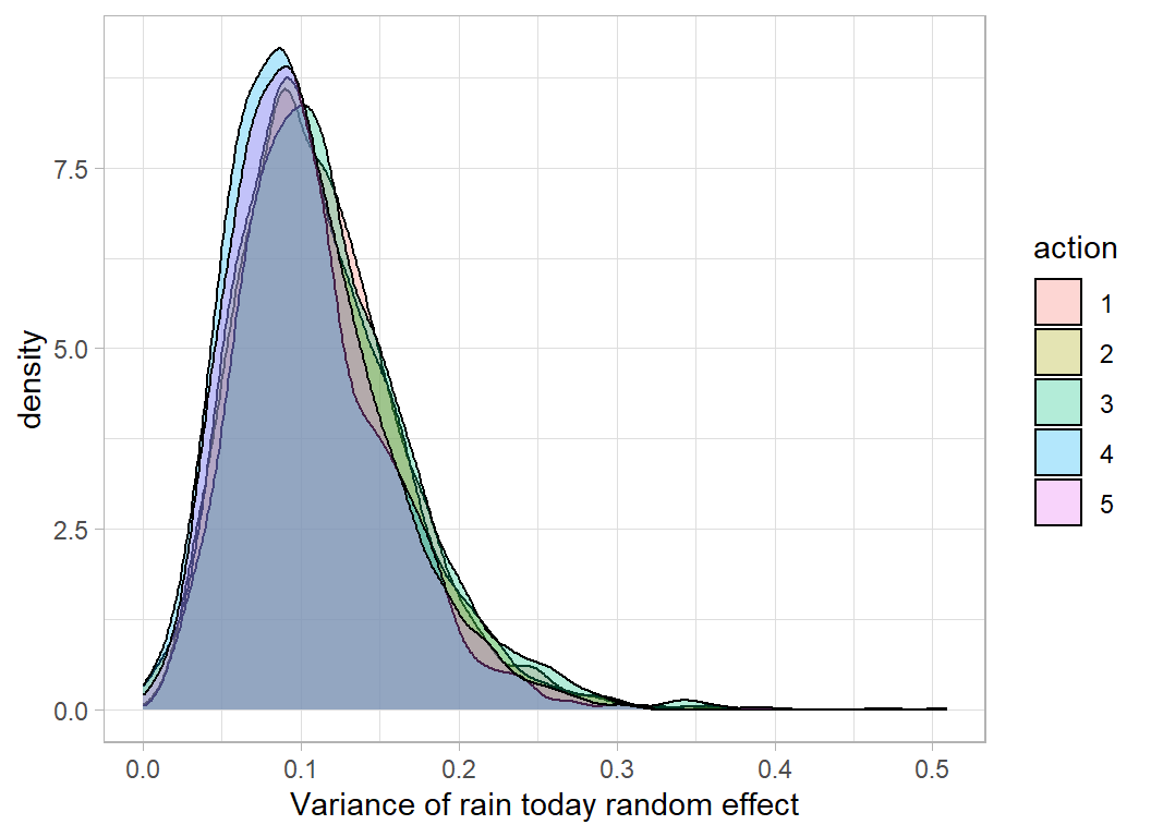
The small differences in the distributions are due in part to the missing values and in part to the MC error of the HMC algorithm. I only ran 2 chains of 1000 post warmup samples on each imputed dataset; longer runs would reduce the MC error and make the effect of the missing values more evident.
Conclusions
Fitting Bayesian hierarchical models is not quick, but the priors have the effect of making the models more stable and they help avoid the convergence failures that are common in likelihood analyses.
Although I have skipped the detail in this post, it is vitally important to inspect the chains produced by a Bayesian analysis to assure yourself that the algorithm really has converged. Failure of a likelihood analysis is fairly clear cut, but failure of a Bayesian analysis is much harder to detect.
A simple mixed model assumes that the 49 cities provide independent samples of the weather in Australia, which of course they do not. The weather in Newcastle is much more similar to the weather in neighbouring Sydney than it is to the weather in Darwin or Perth. A better model would incorporate the geography of the country. One way to do this would be to introduce a state variable, so that the hierarchical structure would be day within location within state within country. Australian states are very large, so this approach would not be ideal, but it is simple and it would probably help.
The big gains from having a hierarchical structure are seen when the data on some of the levels are sparse. Imagine, adding a new location with only one week of weather data. The estimates for that locations would be unreliable, but they would be improved by making use of the pattern of data across the other cities. However, when the data are not sparse, very little transfer of information takes place and the hierarchical estimates will be similar to those that would have been obtained from an independent analysis of that city. In this data set of 15,000 observations over 49 locations, there is an average of over 300 days’ data for each location. The within location parameter estimates are well-identified and the extra computation required for a hierarchical model is probably not justified.