Bayesian Sliced 1: Boardgame Ratings
Summary
Background: In episode 1 of the 2021 series of Sliced, the competitors were given two hours to analyse a set of data on boardgames. The aim was to predict the games’ ratings.
My approach: In an earlier post entitled Sliced Episode 1: Boardgame Ratings, I analysed these data using traditional methods. That post describes my data cleaning, feature selection and data exploration. In this analysis, I take those same cleaned data and analyse them using a Bayesian model. As in my original analysis, I use a spline-based regression model to predict the ratings. The Bayesian version is fitted using OpenBUGS called from within R.
Result: The results from the Bayesian model are very similar to those obtained from a spline-based model fitted with mgcv. Inspecting the predictive distributions highlights a weakness in the model that I used previously. An improved model preforms only marginally better.
Conclusion: A Bayesian model is a practical alternative to a traditional approach. Bayesian models give a more complete picture of both the predictions and the certainty of those predictions.
Introduction
In the first episode of Sliced 2021 the contestants were asked to build a model for predicting the ratings given to boardgames by the website https://boardgamegeek.com/. Model evaluation was by root mean square error (RMSE).
I analysed these data in an earlier post called Spliced Episode 1: Boardgames. That post describes data cleaning, feature extraction, data exploration and a spline model fitted using the R package mgcv.
This is the first of a series of posts in which I will re-analyse the Sliced data using Bayesian methods. For this episode, I stay with spline models, but fit them in R with code that calls OpenBUGS.
This post assumes some basic knowledge of Bayesian methods, so if you are not already familiar with Bayesian modelling in R, you might find it helpful to start by reading my methods posts,
- Methods: Introduction to the Bayesian Analyses
- Methods: MCMC algorithms
- Methods: R Software for Bayesian Analysis
- Methods: Assessing MCMC output
In this post I describe three Bayesian models,
- Splines with 5 knots and a vague prior
- Splines with 20 knots and a smoothing prior
- Splines with 20 knots, a smoothing prior and an improved transformation of the geek rating
Describing a Bayesian analysis properly requires an exploration of convergence and a careful summary of the final MCMC simulations. Add the investigation of the predictive distributions and this would make for an exceptionally long post, so I have been forced to omit some of the details. I give a full account of the first analysis, but leave out parts of the other analyses where they would have been repetitive.
Reading the data
I start by reading the clean data and log transforming the response and the continuous predictors, as I did in my earlier non-Bayesian analysis.
# --- set libraries & options ------------------------
library(tidyverse)

theme_set( theme_light())

# --- set home directory -------------------------------
oldHome <- "C:/Projects/kaggle/sliced/s01-e01"
home    <- "C:/Projects/kaggle/sliced/Bayes-s01-e01"

# --- read clean training data ------------------------------
readRDS( file.path(oldHome, "data/rData/clean_train.rds")) %>%
  mutate( geek_rating = log10(geek_rating - 5.5),
          owned       = log10(owned),
          num_votes   = log10(num_votes),
          min_players = log10(min_players),
          max_players = log10(max_players),
          min_time    = log10(min_time),
          max_time    = log10(max_time),
          avg_time    = log10(avg_time)) -> trainDF

# --- print variable names ----------------------------------
names(trainDF)
## [1] "game_id" "names" "min_players" "max_players" "avg_time"
## [6] "min_time" "max_time" "year" "geek_rating" "num_votes"
## [11] "age" "owned" "M1" "M2" "M3"
## [16] "M4" "M5" "M6" "M7" "M8"
## [21] "M9" "M10" "C1" "C2" "C3"
## [26] "C4" "C5" "C6" "C7" "C8"
## [31] "C9" "C10"The training set contains two identifiers (game_id and names), the response (geek_rating), nine continuous predictors (min_players to owned), ten binary predictors derived from the description of the game mechanics (M1 to M10) and ten binary predictors derived from the categorisation of game type (C1 to C10).
The 5 Knot Model
In my first Bayesian models, I have chosen to fit splines for year, num_votes and owned and to use quadratics for the other continuous predictors. A predictor such as age (minimum age to play the game) has a limited range of possible values and does not really justify a spline.
For my first model, I’ll use splines with 5 knots and because the number of knots is small there will be plenty of data between each knot and vague priors will suffice for the model coefficients.
Preparing the data
The predictors are all scaled by subtracting their means and dividing by their standard deviations. Having the predictors on a common scale will ensure that their coefficients are of similar size, which often helps with the convergence of Bayesian algorithms and it makes it easier to set sensible priors.
# --- scaled predictors ------------------------------
trainDF %>%
  select( -game_id, -names, -geek_rating) %>%
  mutate( across( everything(), scale)) %>%
  as.matrix() -> X

# --- scaled response --------------------------------
trainDF %>%
  mutate( geek_rating = scale(geek_rating)) %>%
  pull(geek_rating) %>%
  as.numeric() -> Y
year is in column 6 of the matrix X, num_votes is in column 7 and owned is in column 9. I choose my knots based on quantiles
# --- sets of 5 knots ------------------------------------------
yearKnots  <- quantile(X[,6], probs=c(0.1, 0.3, 0.5, 0.7, 0.9))
voteKnots  <- quantile(X[,7], probs=c(0.1, 0.3, 0.5, 0.7, 0.9))
ownedKnots <- quantile(X[,9], probs=c(0.1, 0.3, 0.5, 0.7, 0.9))

# --- knots for owned as an example ----------------------------
print(ownedKnots)
## 10% 30% 50% 70% 90%
## -1.1593183 -0.5959975 -0.1296044 0.4057671 1.3717000A cubic spline with 5 knots has 8 coefficients (5 for knots + 3 for cubic + 0 as I omit the intercept), so the three splines require a total of 24 coefficients, to which must be added an overall intercept, the two coefficients of each quadratic and the twenty coefficients for binary predictors.
The package splines calculates the design matrix for fitting cubic splines. Below I create a design matrix, S, for all of the terms in the model.
library(splines)

# --- quadratic terms for six predictors --------------------------
S <- matrix(0, nrow=3499, ncol=12)
k <- 0
for( i in c(1:5, 8)) {
   k <- k + 1
   S[, k] <- X[, i]
   k <- k + 1
   S[, k] <- X[, i]*X[, i]
}
# --- splines for three predictors --------------------------------
S <- cbind(S, as.matrix( bs(X[, 6], knots=yearKnots,
                     degree=3,
                     intercept = FALSE) ))
S <- cbind(S, as.matrix( bs(X[, 7], knots=voteKnots,
                     degree=3,
                     intercept = FALSE) ))
S <- cbind(S, as.matrix( bs(X[, 9], knots=ownedKnots,
                     degree=3,
                     intercept = FALSE) ))
# --- 20 binary predictors ----------------------------------------
S <- cbind(S, X[, 10:29])
I have chosen to use cubic(degree 3), basis-spines (bs) without an intercept. Rather than directly fit cubics to the regions between the knots, this method sets up a mathematically equivalent set of basis functions such that the cubic spline curve is created as a linear combination of the basis functions.
Let’s look at the 8 basis functions created for owned. The basis splines depend on the chosen knots plus boundary knots placed automatically at the minimum and maximum of the data.
# --- a range of values for the standardised owned ------------
x <- seq(min(X[, 9]), max(X[, 9]), 0.1)
# --- coefficients of the basis functions ---------------------
SO <- as.matrix( bs(x, knots=ownedKnots,
                     degree=3,
                     intercept = FALSE) )
# --- plot the 8 basis functions ------------------------------
tibble( y = as.numeric(SO),
        x = rep(x, 8),
        f = rep(1:8, each=69)) %>%
  ggplot( aes(x=x, y=y, group=f)) +
  geom_line() +
  geom_vline( xintercept=ownedKnots, lty=2) +
  labs(title = "8 Basis functions for owned",
       x = "Standardised number who own the game",
       y = "Value of the basis function")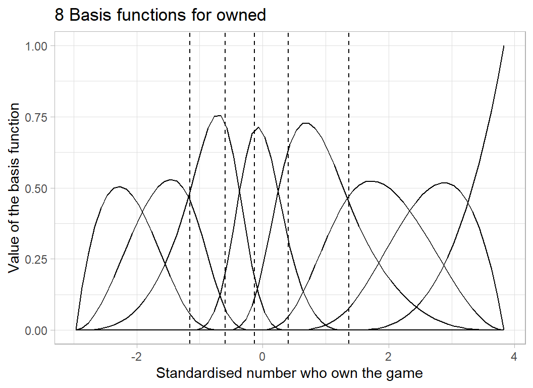
To illustrate how the spline curves are created, I generate some random coefficients and look at the corresponding spline curve.
# --- a random set of coefficients ------------------------
set.seed(8720)
b <- rnorm(8, 0, 0.5)
print(b)
## [1] 0.03183952 -0.19061582 0.02222144 0.80216086 -0.50519207 0.28324566
## [7] 0.09720137 1.30996759# --- plot the implied spline curve -----------------------
tibble( y = SO %*% b,
x = x) %>%
ggplot( aes(x=x, y=y)) +
geom_line() +
geom_vline( xintercept=ownedKnots, lty=2)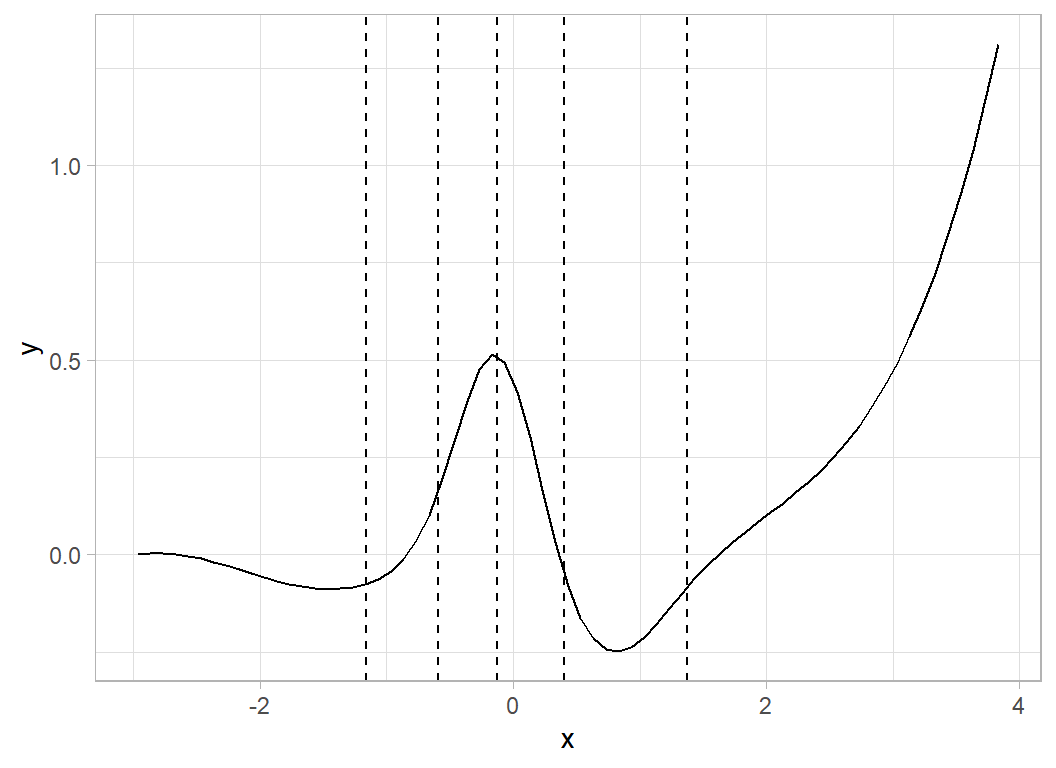
The curve is pinned to zero (there is no intercept) at its lower boundary remains fairly flat (the first random coefficient is close to zero), dips (negative coefficient), rises (coefficient of 0.8), dips again (coefficient of -0.5) and finally rises (coefficient of 1.3).
A Key Step
I have the design matrix, S, for fitting my model, but for Gibbs Sampling to work efficiently, it helps greatly if the columns of S are centred. The idea behind this step is to reduce the correlation between the intercept and the coefficients associated with the columns of S.
Correlation between the intercept and the slope is always a problem in regression but with splines it is particularly acute. Since splines are so flexible, it is easy to compensate for a change in the intercept by making a small change in the spline coefficients. The impact of the high correlation is that the Gibbs Sampler moves very, very slowly across the joint posterior.
Centring reduces the correlation by moving the intercept from the left edge of the data to the centre of the data.
# --- centre all columns of S -------------------------------------
for(i in 1:ncol(S)) {
  S[, i] <- S[, i] - mean(S[, i])
}
Back to the analysis
Now I have all of the data needed for the model, so they are placed in a list ready for passing to OpenBUGS.
# --- place the data in a list to be passed to bugs ---------------
bugsData <- list(S=S, Y=Y)
# --- save the bugs data in an rds file --------------------------
saveRDS( bugsData, file.path(home, "bugs/spline_data.rds"))
The response is in a 3499x1 column vector, Y, and the predictors are in a 3499x56 matrix, S.
Generalised Additive Models
My OpenBUGS code for this model is written to a text file called bugs/spline_model.txt. Here is the content of that file.
model {
  for( i in 1:3499 ) {

    # quadratics for 6 predictors

    quad[i] <- a[1]*S[i, 1] + a[2]*S[i, 2] + a[3]*S[i, 3] +
               a[4]*S[i, 4] + a[5]*S[i, 5] + a[6]*S[i, 6] +
               a[7]*S[i, 7] + a[8]*S[i, 8] + a[9]*S[i, 9] +
               a[10]*S[i, 10] + a[11]*S[i, 11] + a[12]*S[i, 12]

    # spline for year

    sYr[i] <- b[1]*S[i, 13] + b[2]*S[i, 14] + b[3]*S[i, 15] +
              b[4]*S[i, 16] + b[5]*S[i, 17] + b[6]*S[i, 18] +
              b[7]*S[i, 19] + b[8]*S[i, 20]

    # spline for num_votes

    sVo[i] <- b[ 9]*S[i, 21] + b[10]*S[i, 22] + b[11]*S[i, 23] +
              b[12]*S[i, 24] + b[13]*S[i, 25] + b[14]*S[i, 26] +
              b[15]*S[i, 27] + b[16]*S[i, 28]

    # spline for owned

    sOw[i] <- b[17]*S[i, 29] + b[18]*S[i, 30] + b[19]*S[i, 31] +
              b[20]*S[i, 32] + b[21]*S[i, 33] + b[22]*S[i, 34] +                          b[23]*S[i, 35] + b[24]*S[i, 36]

    # game mechanism

    mec[i] <- c[1]*S[i, 37] + c[2]*S[i, 38] + c[3]*S[i, 39] +
              c[4]*S[i, 40] + c[5]*S[i, 41] + c[6]*S[i, 42] +
              c[7]*S[i, 43] + c[8]*S[i, 44] + c[9]*S[i, 45] +
              c[10]*S[i, 46]

    # game category

    cat[i] <- c[11]*S[i, 47] + c[12]*S[i, 48] + c[13]*S[i, 49] +
              c[14]*S[i, 50] + c[15]*S[i, 51] + c[16]*S[i, 52] +
              c[17]*S[i, 53] + c[18]*S[i, 54] + c[19]*S[i, 55] +
              c[20]*S[i, 56]

    # combined linear predictor

    mu[i] <- a0 + quad[i] + sYr[i] + sVo[i] + sOw[i] + mec[i] + cat[i]

    # distribution of the game rating

    Y[i] ~ dnorm(mu[i], tau)
  }

# Priors

  # intercept

  a0 ~ dnorm(0.0, 0.01)

  # quadratics

  for( j in 1:12) {
    a[j] ~ dnorm(0, 0.01)
  }
  # spline coefficients

  for(j in 1:24 ) {
    b[j] ~ dnorm(0, 0.01)
  }

  # categorical predictors

  for(j in 1:20 ) {
    c[j] ~ dnorm(0, 0.01)
  }

  # residual precision

  tau ~ dgamma(2, 1)
  }
I am fitting a linear regression with constant variance and 56 predictors. I place priors on the coefficients that are zero centred and have a precision of 0.01. This precision is equivalent to a variance of 100 or a standard deviation of 10. The net result is that I am expecting all of the coefficients to be in the range -20 to 20. Given that the scales have been standardised, this seems sufficiently vague to me.
The prior on the precision of the residuals, tau, has a mean of 2 (2/1) and a standard deviation of 1.4 (sqrt(2)/1). A precision of 2 is equivalent to a variance of 0.5. Since Y is standardised to have a variance of 1, a residual variance of 0.5 would imply that the regression equation explains 50% of the variance, which again seems reasonable to me.
Arguably, since I know that tau will be greater than 1, a gamma prior is inappropriate and I ought to use a truncated distribution. While this is true, a gamma prior leads to a gamma posterior for tau, which greatly improves the speed of the sampling and since tau is estimated from over three thousand observations, I anticipate that a truncated prior would have little impact.
Fitting the model
I have no idea how well OpenBUGS with perform with this model, so I am forced to make guesses. I will run three chains, each with a burn-in of 2000 iterations and a run length of a further 1000.
To start with I create a tibble that contains all of the details needed to control my three chains.
# --- create the analysis tibble ---------------------------------
set.seed(1782)
tibble(
        model   = rep( file.path(home, "bugs/spline_model.txt"), 3),
        data    = rep( file.path(home, "bugs/spline_data.rds"), 3),
        niter   = rep(3000, 3),
        nburnin = rep(2000, 3),
        thin    = rep(1, 3),
        seed   = c(3, 4, 5),
        inits   = list(
                    list(a0  = rnorm(1, 0, 0.25),
                         a   = rnorm(12, 0, 0.25),
                         b   = rnorm(24, 0, 0.25),
                         c   = rnorm(20, 0, 0.25),
                         tau = rgamma(1, shape=5, rate=1)),
                    list(a0  = rnorm(1, 0, 0.25),
                         a   = rnorm(12, 0, 0.25),
                         b   = rnorm(24, 0, 0.25),
                         c   = rnorm(20, 0, 0.25),
                         tau = rgamma(1, shape=5, rate=1)),
                    list(a0  = rnorm(1, 0, 0.25),
                         a   = rnorm(12, 0, 0.25),
                         b   = rnorm(24, 0, 0.25),
                         c   = rnorm(20, 0, 0.25),
                         tau = rgamma(1, shape=5, rate=1)) ),
        wDir    = paste(
          file.path(home, "temp/chain"), 1:3, sep=""),
        sims    = paste(
          file.path(home, "data/dataStore/spline_1_"), 1:3,".rds", sep="")
  ) %>%
  print() -> bugsRunDF
## # A tibble: 3 x 9
## model data niter nburnin thin seed inits wDir sims
## <chr> <chr> <dbl> <dbl> <dbl> <dbl> <list> <chr> <chr>
## 1 C:/Projects/kaggle/s~ C:/P~ 3000 2000 1 3 <named list> C:/P~ C:/P~
## 2 C:/Projects/kaggle/s~ C:/P~ 3000 2000 1 4 <named list> C:/P~ C:/P~
## 3 C:/Projects/kaggle/s~ C:/P~ 3000 2000 1 5 <named list> C:/P~ C:/P~ # --- save as permanent record of the analysis ---------------------
saveRDS( bugsRunDF, file.path(home, "data/dataStore/spline_1_table.rds")) To enable me to run the chains in parallel, I place the code for a single chain in a function.
# --- function to run a single chain ------------------------------
# arguments correspond to the columns of the analysis tibble
#
# returns
#    nothing .. results written to rds files
#
run_bugs <- function(model, data, niter, nburnin, thin, seed,
                          inits, wDir, sims)
{
  library(R2OpenBUGS)

  # --- OpenBUGS executable
  obExe   <- "C:/Software/OpenBUGS/OpenBUGS323/OpenBUGS.exe"

  # --- call to bugs() ---------------------------------------------
  bugs( data = readRDS(data),
        inits = list(inits),
        parameters = c("a0", "a", "b", "c", "tau"),
        model.file = model,
        n.chains = 1,
        n.iter = niter,
        n.burnin = nburnin,
        n.thin = thin,
        digits = 5,
        codaPkg = FALSE,
        bugs.seed = seed,
        OpenBUGS = obExe,
        working.directory = wDir
  ) %>%
  # --- save the returned bugs object -----------------------------
     saveRDS(sims)
}
I need to keep the three parallel chains isolated from one another, so I create three working directories.
# --- Create 3 working directories ---------------------------------
for( i in 1:3 ) {
  # --- address of the working directory ---------------------------
  folder <- file.path( home, paste("temp/chain", i, sep=""))
  # --- delete it if it already exists -----------------------------
  if( dir.exists(folder)) {
    unlink(folder, recursive=TRUE)
  }
  # --- create the working directory -------------------------------
  dir.create(folder)
}
Now the three chains can be run on separate cores using the furrr package.
library(furrr)
# --- run three independent R sessions --------------
plan(multisession, workers=3)

# --- run the chains in parallel --------------------
bugsRunDF %>%
  future_pwalk(run_bugs) %>%
  system.time()

# --- switch back to sequential processing ----------
plan(sequential)
This run took 14 minutes on my ancient desktop.
In my methods posts, I describedmy functions for extracting the simulations into a data frame. Here, I use bayes_to_df().
library(MyPackage)

# --- read the simulations --------------------------------
bayes_to_df(bugsRunDF$sims) %>%
  print() -> simDF
## # A tibble: 3,000 x 61
## chain iter a0 a_1 a_2 a_3 a_4 a_5 a_6 a_7
## <fct> <int> <dbl> <dbl> <dbl> <dbl> <dbl> <dbl> <dbl> <dbl>
## 1 1 1 -0.00482 0.00389 0.00294 -0.0841 0.0289 -0.199 -0.104 0.136
## 2 1 2 -0.00403 -0.00963 0.0134 -0.0857 0.0348 -0.285 -0.137 0.164
## 3 1 3 0.00133 0.0103 0.0172 -0.0785 0.0288 -0.227 -0.158 0.160
## 4 1 4 0.000331 -0.00897 0.0146 -0.0848 0.0345 -0.173 -0.0926 0.119
## 5 1 5 -0.00206 -0.00268 0.00999 -0.0790 0.0269 -0.166 -0.190 0.139
## 6 1 6 -0.00827 -0.00548 0.0108 -0.0800 0.0326 -0.164 -0.113 0.142
## 7 1 7 -0.00492 -0.00782 0.0118 -0.0802 0.0276 -0.175 -0.0979 0.155
## 8 1 8 0.00176 -0.00975 0.0108 -0.0872 0.0297 -0.0777 -0.120 0.105
## 9 1 9 -0.00184 -0.00463 0.0127 -0.0784 0.0361 -0.124 -0.0634 0.0779
## 10 1 10 -0.00173 -0.00670 0.0112 -0.0979 0.0366 -0.145 -0.116 0.129
## # ... with 2,990 more rows, and 51 more variables: a_8 <dbl>, a_9 <dbl>,
## # a_10 <dbl>, a_11 <dbl>, a_12 <dbl>, b_1 <dbl>, b_2 <dbl>, b_3 <dbl>,
## # b_4 <dbl>, b_5 <dbl>, b_6 <dbl>, b_7 <dbl>, b_8 <dbl>, b_9 <dbl>,
## # b_10 <dbl>, b_11 <dbl>, b_12 <dbl>, b_13 <dbl>, b_14 <dbl>, b_15 <dbl>,
## # b_16 <dbl>, b_17 <dbl>, b_18 <dbl>, b_19 <dbl>, b_20 <dbl>, b_21 <dbl>,
## # b_22 <dbl>, b_23 <dbl>, b_24 <dbl>, c_1 <dbl>, c_2 <dbl>, c_3 <dbl>,
## # c_4 <dbl>, c_5 <dbl>, c_6 <dbl>, c_7 <dbl>, c_8 <dbl>, c_9 <dbl>, ...Usually, the intercept and the precision are the most difficult parameters to estimate, so I check them first using my trace_plot() function, which is also described in my methods posts.
# --- trace plot of the intercept ------------------------------
trace_plot(simDF, a0) +
  labs(title = "Intercept")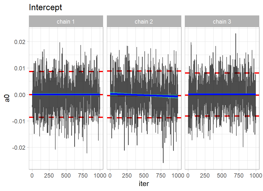
# --- trace plot of the residual standard deviation ------------
simDF %>%
  mutate( sigma = 1/sqrt(tau) ) %>%
  trace_plot(sigma) +
  labs( title = "Residual Standard Deviation")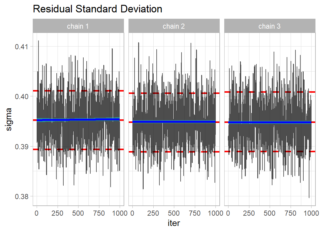
The mixing within chains is quite good, so locally the chains are moving freely across the posterior. The agreement between the chains suggests that they have converged to the same solution.
A good measure of performance that is easy to apply to all parameters is the Gelman-Rubin-Brooks statistic, Rhat. This can be obtained from the coda package. So I put the simulations into coda format.
library(coda)
# --- coda format of the 3 OpenBUGS chains ------------------------
bugsCoda <- mcmc.list( mcmc( simDF %>%
                                filter( chain == 1) %>%
                                select(-chain, -iter)),
                       mcmc( simDF %>%
                                filter( chain == 2) %>%
                                select(-chain, -iter)),
                       mcmc( simDF %>%
                                filter( chain == 3) %>%
                                select(-chain, -iter)) )

# --- Gelman-Rubin-Brooks statistics ------------------------------
gelman.diag(bugsCoda)
## Potential scale reduction factors:
##
## Point est. Upper C.I.
## a0 1.002 1.007
## a_1 1.000 1.002
## a_2 1.003 1.011
## a_3 1.000 1.002
## a_4 1.001 1.002
## a_5 1.950 3.251
## a_6 1.653 2.606
## a_7 1.976 3.285
## a_8 1.520 2.310
## a_9 1.751 2.852
## a_10 1.694 2.698
## a_11 1.004 1.005
## a_12 1.004 1.017
## b_1 1.005 1.021
## b_2 1.005 1.015
## b_3 1.021 1.075
## b_4 1.014 1.034
## b_5 1.033 1.107
## b_6 1.020 1.064
## b_7 1.026 1.083
## b_8 1.018 1.058
## b_9 1.046 1.138
## b_10 1.037 1.096
## b_11 1.054 1.158
## b_12 1.057 1.154
## b_13 1.095 1.286
## b_14 1.042 1.088
## b_15 1.164 1.494
## b_16 1.005 1.009
## b_17 1.442 2.142
## b_18 1.446 2.148
## b_19 1.712 2.752
## b_20 1.675 2.652
## b_21 1.775 2.880
## b_22 1.513 2.304
## b_23 1.397 2.042
## b_24 1.026 1.062
## c_1 1.005 1.017
## c_2 1.001 1.004
## c_3 1.002 1.007
## c_4 0.999 1.000
## c_5 1.000 1.001
## c_6 1.002 1.007
## c_7 0.999 0.999
## c_8 1.000 1.003
## c_9 1.000 1.004
## c_10 1.000 1.001
## c_11 1.012 1.044
## c_12 1.034 1.118
## c_13 1.013 1.045
## c_14 1.002 1.007
## c_15 1.001 1.006
## c_16 1.014 1.047
## c_17 0.999 1.000
## c_18 1.000 1.000
## c_19 1.003 1.010
## c_20 1.003 1.013
## tau 1.005 1.020
## deviance 1.005 1.018
##
## Multivariate psrf
##
## 1.84The point estimates of Rhat are below 1.05 for most parameters, suggesting good agreement between chains. The noticeable exceptions are the parameters of the third spline, which describes the pattern for the number of people who own the game. It appear that more iterations would be needed for this curve to stabilise. Given the short run that was used to create these simulations, I am more encouraged by the overall performance than discouraged by the spline for owned.
Finally. I look at the shapes of the shapes of the three spline curves based on the posterior mean estimates of the coefficients.
# --- Simple function to plot a spline curve ---------------
# arguments
#    x  ... range of values for plotting
#    knots ... positions of the knots
#    coef  ... model coefficients
#
plot_spline <- function(x, knots, coef) {
  S <- as.matrix( bs(x, knots=knots,
                     degree=3,
                     intercept = FALSE) )
  y <- as.numeric(S %*% b)

  tibble( x=x, y=y) %>%
    ggplot( aes(x=x, y=y)) +
    geom_line() +
    geom_vline( xintercept=knots, lty=2)
}

# --- place 24 spline coefficients in matrix ---------------
simDF %>%
  select( starts_with("b")) %>%
  as.matrix() -> splCoef

# --- 'Average' spline curve for Year ----------------------
x <- seq(min(X[, 6]), max(X[, 6]), 0.1)
b <- apply(splCoef[, 1:8], 2, mean)
plot_spline(x, yearKnots, b) +
  labs(x="Standardised Year")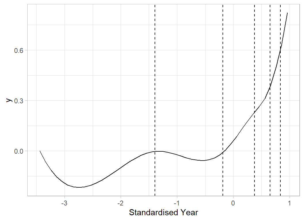
# --- 'Average' spline curve for Votes ---------------------
x <- seq(min(X[, 7]), max(X[, 7]), 0.1)
b <- apply(splCoef[, 9:16], 2, mean)
plot_spline(x, voteKnots, b) +
  labs(x="Standardised Number of Votes")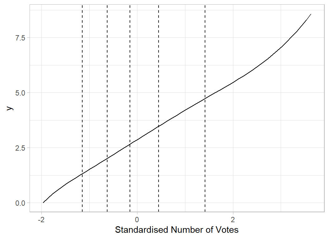
# --- 'Average' spline curve for Owned ---------------------
x <- seq(min(X[, 9]), max(X[, 9]), 0.1)
b <- apply(splCoef[, 17:24], 2, mean)
plot_spline(x, ownedKnots, b) +
  labs(x="Standardised Number who Own the Game")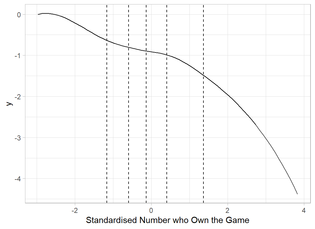
I could run a longer chain for this model in order to improve the estimation, but since it was only intended as a preliminary investigation, I will skip that stage and move to the model with 20 knots.
The 20 Knot Model
In my first model, I used 5 knots for each spline and I placed the knots using quantiles of the data. This choice was completely arbitrary and leaves open the question of whether a different choice of knots might have led to a better model.
I could try different sets of knots until I hit on a curve that looks good by eye, but this would be a terrible idea,
* The process would be very time consuming
* The chosen curve would not be reproducible
* Other data analysts would not be able to judge or criticise my choice
* I would use the same data to fit the model and to guide my ‘by-eye’ model choice, which would probably result in over-fitting
One solution is use so many knots that the actual number or placement hardly matters, but in that case, it would be possible for the curve to be extremely wiggly. When the coefficients for one strip are similar to those in the next strip the spline curve will not be able to wiggle. What I need is a large number of knots together with a prior that says that I anticipate that successive spline coefficients will be similar.
I’ve chosen to have 20 knots placed at evenly spread quantiles, which means 23 coefficients for each spline. year takes integer values and is dominated by values after 2000. When the quantile function is used, there are only 18 unique values, so I end with 18 knots for this predictor.
# --- target number of knots, K --------------------------------
K <- 20
# --- sequence of quantiles ------------------------------------
pr <- seq( 1/(2*K), 1 - 1/(2*K), length=K)
# --- sets of knots --------------------------------------------
yearKnots  <- unique(quantile(X[,6], probs=pr))
nYearKnots <- length(yearKnots)
voteKnots  <- unique(quantile(X[,7], probs=pr))
nVoteKnots <- length(voteKnots)
ownedKnots <- unique(quantile(X[,9], probs=pr))
nOwnedKnots <- length(ownedKnots)

# --- numbers of unique knots ----------------------------------
print( c(nYearKnots, nVoteKnots, nOwnedKnots))
## [1] 18 20 20The design matrix is created and centred, just as it was for the 5 knot model.
My bugs code also resembles that for the 5 knot model. I just give the code for the expanded year spline, this has 21 coefficients (18 knots + 3).
# the spline curve for year
sYr[i] <- b[ 1]*S[i,13] + b[ 2]*S[i,14] + b[ 3]*S[i,15] + b[ 4]*S[i,16] +
          b[ 5]*S[i,17] + b[ 6]*S[i,18] + b[ 7]*S[i,19] + b[ 8]*S[i,20] +
          b[ 9]*S[i,21] + b[10]*S[i,22] + b[11]*S[i,23] + b[12]*S[i,24] +
          b[13]*S[i,25] + b[14]*S[i,26] + b[15]*S[i,27] + b[16]*S[i,28] +
          b[17]*S[i,29] + b[18]*S[i,30] + b[19]*S[i,31] + b[20]*S[i,32] +
          b[21]*S[i,33]

........................................

# the smoothing prior on the coefficients
b[1] ~ dnorm(0, 0.01)
for(j in 2: 21 ) {
  b[j] ~ dnorm(b[j-1], eta1)
}
eta1 ~ dgamma(1, 0.04)
My prior on the spline coefficients for year says that each spline coefficient is a small deviation from the previous one with the deviations having a precision eta1. The eta has an expected precision of 25, so the variance is 0.04 and the standard deviation is 0.2. My prior on eta leans towards small deviations but is vague enough that their is scope for the data to influence the wiggliness.
The code for fitting the model is essentially the same as for the preliminary model, so I do not repeat it. I run 3 chains of length 10,000 of which the first 5,000 iterations were discarded as the burn-in. The code took almost exactly 2 hours to run.
Convergence is reasonable although I do not show details. It is in the nature of a Bayesian analysis that one would always like a few more iterations, but I judged that my run length was an acceptable compromise.
Here is a plot that looks at the 21 spline coefficients for year. The plot shows the median and 95% credible intervals and demonstrates how the coefficients change gradually.
library(coda)
library(MyPackage)

# --- extract and combine --------------------------------------
simDF <- NULL
for( i in 1:3 ) {
  rf       <- file.path( home,
                         paste("data/dataStore/finalSplineP0", i, ".rds",sep=""))
  simDF <- bind_rows( simDF,
                      bugs_to_df( readRDS(rf)) %>% mutate( chain = i) )
}
# --- convert chain into a factor -------------------------------
simDF %>%
  mutate( chain = factor(chain)) -> simDF
# --- show the tibble -------------------------------------------
print(simDF)
## # A tibble: 15,000 x 106
## chain iter a0 a_1 a_2 a_3 a_4 a_5 a_6 a_7
## <fct> <int> <dbl> <dbl> <dbl> <dbl> <dbl> <dbl> <dbl> <dbl>
## 1 1 1 0.00200 5.19e-3 0.00642 -0.0794 0.0300 -0.121 -0.0936 0.082
## 2 1 2 -0.00907 -1.99e-3 0.0167 -0.0798 0.0392 -0.101 -0.144 0.0934
## 3 1 3 0.00177 -1.39e-2 0.00988 -0.0698 0.0339 -0.139 -0.0788 0.117
## 4 1 4 0.00944 -6.98e-3 0.0114 -0.0805 0.0201 -0.0595 -0.0783 0.0499
## 5 1 5 0.00489 -5.09e-4 0.0160 -0.0882 0.0359 -0.209 -0.161 0.161
## 6 1 6 0.000593 -6.28e-3 0.00603 -0.0764 0.0348 -0.0818 -0.103 0.0807
## 7 1 7 0.00187 -6.25e-3 0.0185 -0.0932 0.0219 -0.166 -0.164 0.146
## 8 1 8 -0.00762 -1.57e-2 0.00259 -0.0774 0.0313 -0.00532 -0.183 0.104
## 9 1 9 0.0113 -1.05e-3 0.0162 -0.0797 0.0299 -0.157 -0.122 0.131
## 10 1 10 -0.00707 1.46e-4 0.00842 -0.0839 0.0295 -0.0702 -0.135 0.0751
## # ... with 14,990 more rows, and 96 more variables: a_8 <dbl>, a_9 <dbl>,
## # a_10 <dbl>, a_11 <dbl>, a_12 <dbl>, b_1 <dbl>, b_2 <dbl>, b_3 <dbl>,
## # b_4 <dbl>, b_5 <dbl>, b_6 <dbl>, b_7 <dbl>, b_8 <dbl>, b_9 <dbl>,
## # b_10 <dbl>, b_11 <dbl>, b_12 <dbl>, b_13 <dbl>, b_14 <dbl>, b_15 <dbl>,
## # b_16 <dbl>, b_17 <dbl>, b_18 <dbl>, b_19 <dbl>, b_20 <dbl>, b_21 <dbl>,
## # b_22 <dbl>, b_23 <dbl>, b_24 <dbl>, b_25 <dbl>, b_26 <dbl>, b_27 <dbl>,
## # b_28 <dbl>, b_29 <dbl>, b_30 <dbl>, b_31 <dbl>, b_32 <dbl>, b_33 <dbl>, ...# --- convert results to code format ----------------------------
bugsCoda <- mcmc(simDF %>% select(-chain, -iter))
# --- use code function summary() to obtain the quantiles -------
summary(bugsCoda)[2] %>%
as.data.frame() %>%
as_tibble(rownames="term") %>%
mutate( term = str_replace(term, "_", "")) %>%
# --- extract coefficients for the year spline ----------------
slice( 14:34 ) %>%
mutate( term=factor(term, levels=paste("b", 1:21, sep=""))) %>%
# --- plot medians and 95% CrI --------------------------------
ggplot( aes(x=term, y=quantiles.50.)) +
geom_point() +
geom_errorbar( aes(ymin=quantiles.2.5.,
ymax=quantiles.97.5.), width=0.2) +
labs(title = "Spline Coefficients for Year",
y = "Median Coefficient & 95% CrI")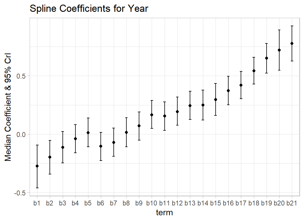
The Predictive Distribution
For illustration, I look at some predictive distributions for a single individual in the training set. As usual I embed the calculation in a function that is given in the Appendix. I start by looking at the results for row 1, a game called Hecatomb with a geek rating of 5.70.
The first plot shows the predictive distribution of the transformed and scaled rating, on this scale Hecatomb scored -1.02 meaning that its score of 5.70 placed it in the bottom 20% of games.
The predictive distribution is simulated, so a seed is set for reproducibility.
set.seed(8118)
# --- Predictive Distribution for hecatomb ------------------
pred_dist(as.matrix(simDF %>% select(-iter, -chain)),
          simDF$tau,
          as.numeric(S[1, ]),
          Y[1])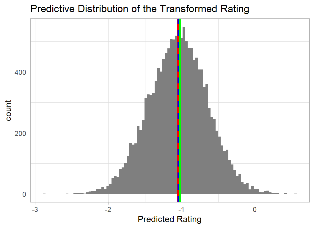
The predictive distribution tells us that the model anticipates a transformed rating between 0 and -2 with the most likely value being just below -1. The mean of the distribution (red) is very close to the true value (green).
The blue dashed line shows the prediction obtained using the posterior means of the coefficients. The importance of this is that it is much quicker to calculate this prediction, as it does not depend on first simulating the predictive distribution.
Performance is clearer if the scaling and transformation are reversed and the predictive distribution is viewed on the original 0-10 scale. I use a function inv_trans_pred_dist() given in the appendix.
The interpretation is unaffected but the plot is easier to understand.
set.seed(8118)
inv_trans_pred_dist(as.matrix(simDF %>% select(-iter, -chain)),
          simDF$tau,
          as.numeric(S[1, ]),
          Y[1])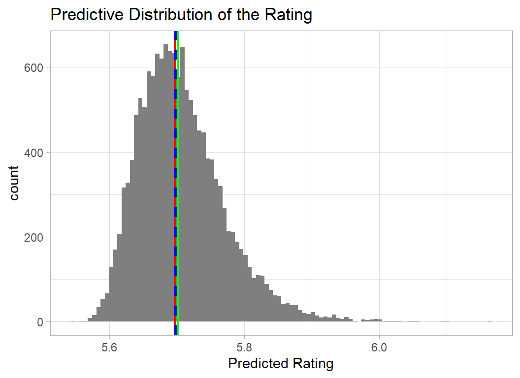
Game 1 is one of the least popular games, so I also look at the predictive distribution of one of the most popular. I’ve chosen row 2053 a game called Gaia Project, which has a rating of 8.00. I show the distribution on the original (0,10) scale.
set.seed(8118)
inv_trans_pred_dist(as.matrix(simDF %>% select(-iter, -chain)),
          simDF$tau,
          as.numeric(S[2053, ]),
          Y[2053])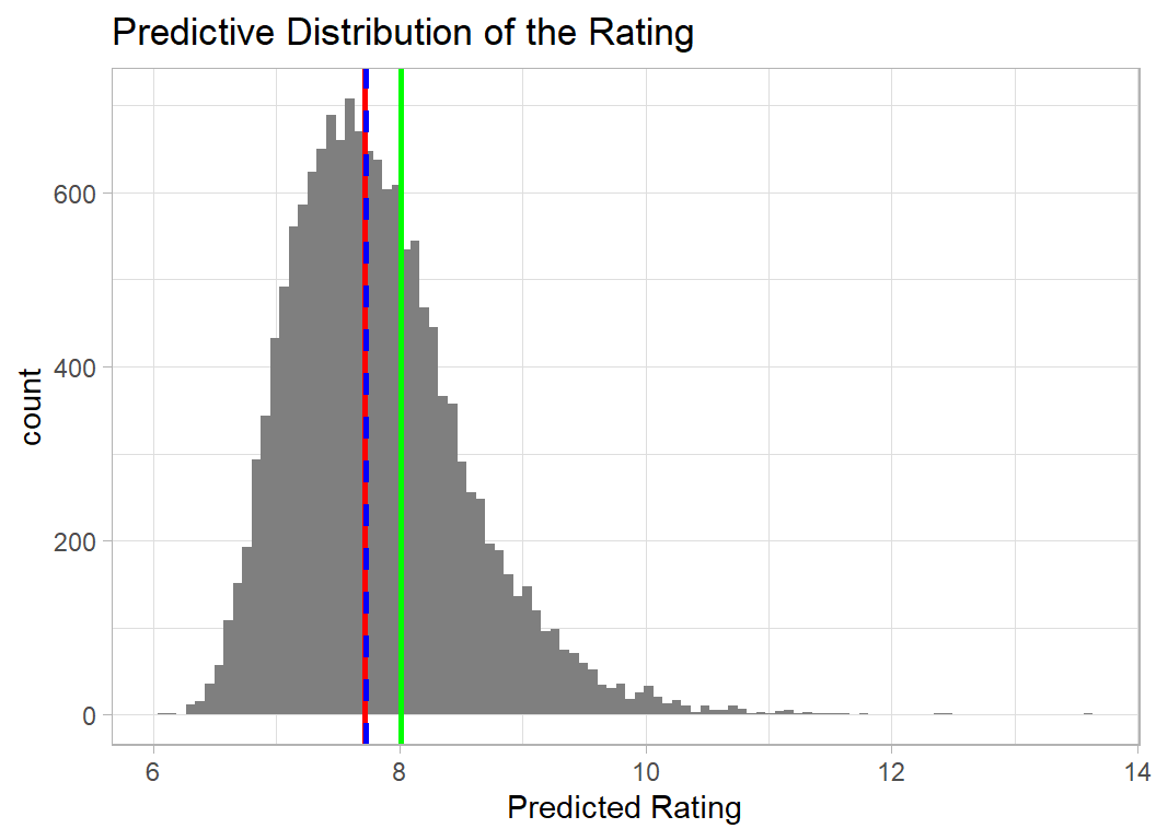
Unfortunately, the model places a small probability on the rating being over 10, which by definition is impossible. It probably makes little difference, but it is somewhat dissatisfying to use a model that makes impossible predictions even if such predictions are rare.
Final 20 knot Model
To ensure that predictions are never over 10, I re-ran the 20 knot model using a different transformation of the geek rating. The logit-style transformation ensures that all predictions back-transform to a value in the range (5.5, 10).
# --- read clean training data ------------------------------
readRDS( file.path(oldHome, "data/rData/clean_train.rds")) %>%
  mutate( geek_rating = log10((geek_rating - 5.5)/(10.0 - geek_rating)),
          owned       = log10(owned),
          num_votes   = log10(num_votes),
          min_players = log10(min_players),
          max_players = log10(max_players),
          min_time    = log10(min_time),
          max_time    = log10(max_time),
          avg_time    = log10(avg_time)) -> trainDF
Here is the new predictive distribution for Gaia Project.
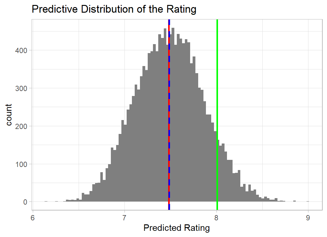
The apparent increase in the difference between the prediction and the actual rating of 8, is partly a reflection of the change in scale of the graph and partly a result of a lower mean when there are no predictions over 10.
Submission
I’ll make my submission based on the blue lines for the new transformation. This involves taking the average of the posterior distributions of each coefficient and predicting using those point estimates.
First I read the test data
# --- read the test data -------------------------------------
readRDS( file.path(oldHome, "data/rData/clean_test.rds")) %>%
  mutate( owned       = log10(owned),
          num_votes   = log10(num_votes),
          min_players = log10(min_players),
          max_players = log10(max_players),
          min_time    = log10(min_time),
          max_time    = log10(max_time),
          avg_time    = log10(avg_time)) -> testDF
Next I scale it using the mean and standard deviation of the training data. I do this with my own scaling function, myScale
# --- scaled predictors ------------------------------
myScale <- function(col) {
  trainDF %>%
    summarise( m = mean({{col}}),
               s = sd({{col}}),
               .groups="drop"
               ) -> statDF
  return( (col-statDF$m)/statDF$s)
}

# --- scale and write as a matrix --------------------
testDF %>%
  select( -game_id, -names) %>%
  mutate( across( everything(), myScale)) %>%
  as.matrix() -> XT
Now I calculate the splines for the test set values of each continuous predictor, saving them in the design matrix ST. Because the basis functions depend on both my choice of knots and the boundaries of the data, I supplement the data with extra points.
Finally I build up the prediction from the intercept and the terms in the linear predictor.
# --- average simulated regression coefficients ----------
simDF %>%
  select( 4:102 ) %>%
  summarise( across(everything(), mean)) %>%
  as.numeric() -> cf

# --- estimate of the mean scaled rating -----------------
mu <- as.numeric( mean(simDF$a0) + ST %*% cf )

# --- reverse the transformations ------------------------
pred <- mean(trainDF$geek_rating) + sd(trainDF$geek_rating) * mu
pred <- (10 ^ (pred + 1) + 5.5)/(10 ^ pred + 1)

# --- show prediction for test set game 1 ----------------
pred[1]
## [1] 7.736849Now I place the predictions in a file using the Sliced format.
# --- create a submission file -----------------------
testDF %>%
  mutate( geek_rating = pred ) %>%
  select( game_id, geek_rating) %>%
  write_csv( file.path(home, "temp/submission.csv"))
When these predictions were submitted, they scored 0.172 on the private leaderboard, good enough for a respectable 8th place.
In my original (non-Bayesian) submission I scored 0.169 with a model that used the transformation of geek_rating that did not impose an upper bound of 10, but which had splines for all of the continuous predictors fitted with the package mgcv.
What this example shows
This is the first of my attempts to re-analyse the Sliced datasets using Bayesian models. For these data, the Bayesian analysis produces predictions that are very close to those that I obtained previously. Despite the size of this dataset, Bayesian computation is still just about feasible, with the final model taking 2 hours to fit. Computation time did deter me from using splines for all of the continuous predictors, although there are other grounds for not using splines with, for example, age which only takes integer values in the range 2 to 18.
My prior on the coefficients of the B-splines penalises values that fluctuate wildly and so limits the wiggliness of the final curve. It is not obvious to me how the similarity of the coefficients relates to the degree of wiggle and so it was not easy to decide what prior to place on the deviations. The sizes of the deviations are largely constrained by the data, so that you do not get curves that are smooth over most of their range, but then have an isolated wiggle. Ideally, more thought should go into this prior. mgcv uses a penalty based on the second derivatives, effectively constraining the changes in the coefficients, rather than their values; this approach could also be used in a Bayesian model.
Looking at predictive distributions rather than point predictions conveys much more information and in this example it highlighted a weakness in my original transformation of geek_rating. This was easily rectified, although the improvement has little impact on performance.
The example illustrates both the strengths and weaknesses of Bayesian analysis. Here are the pros and cons that seem important to me
Disadvantages
- longer computation time
- specifying priors is not easy
- there is more to check
Advantages
- posterior distributions are more informative than point estimates
- predictive distributions are more informative than point predictions
- priors provide a logical basis for penalisation
- the model and its assumptions are more transparent
Of these factors, the most important is probably the computation time. It is hard to justify a Bayesian analysis when the computational burden restricts one’s choice of model.
Appendix
Functions for displaying the predictive distribution
pred_dist <- function(sims, tau, s, y) {
  dim(sims)
  length(s)
  mu <- sims[,1] + sims[,2:100] %*% s
  yStar <- rnorm(nrow(sims), mu, 1/sqrt(tau))
  yMean <- mean(sims[,1]) + apply(sims[,2:100], 2, mean) %*% s
  yPredMean <- mean(yStar)
  tibble( x = yStar) %>%
    ggplot( aes(x=x)) +
    geom_histogram( bins=100, fill="grey50") +
    geom_vline( xintercept=y, colour="green", size=1) +
    geom_vline( xintercept=yMean, colour="red", size=1, lty=1) +
    geom_vline( xintercept=yPredMean, colour="blue", size=1, lty=2) +
    labs(x = "Predicted Rating",
         title= "Predictive Distribution of the Transformed Rating")
}

inv_trans <- function(y) {
  y <- sd(trainDF$geek_rating) * y + mean(trainDF$geek_rating)
  y <- 5.5 + 10 ^ y
  return(y)
}

inv_trans_pred_dist <- function(sims, tau, s, y) {
  mu <- sims[,1] + sims[,2:100] %*% s
  yStar <- rnorm(nrow(sims), mu, sd=1/sqrt(tau))
  yPredMean <- mean(yStar)
  yMean <- mean(sims[,1]) + apply(sims[,2:100], 2, mean) %*% s
  yStar <- inv_trans(yStar)
  yMean <- inv_trans(yMean)
  yPredMean <- inv_trans(yPredMean)
  tibble( x = yStar) %>%
    ggplot( aes(x=x)) +
    geom_histogram( bins=100, fill="grey50") +
    geom_vline( xintercept=inv_trans(y), colour="green", size=1) +
    geom_vline( xintercept=yMean, colour="red", size=1, lty=1) +
    geom_vline( xintercept=yPredMean, colour="blue", size=1, lty=2) +
    labs(x = "Predicted Rating",
         title= "Predictive Distribution of the Rating")
}