Bayesian Sliced 5: Airbnb Price Prediction
Summary:
Background: In episode 5 of the 2021 series of Sliced, the competitors were given two hours in which to analyse a set of data on Airbnb properties in New York City. The aim was to predict the price per night.
My approach: I analyse the data using Bayesian additive regression trees (BART) fitted using the BART package.
Result: Even with over 300 potential predictors, the BART models fit remarkably quickly, although the default burn-in proved insufficient. The results are comparable with those obtained with XGBoost. The choice of priors can alter the predictors that are used without changing the predictive performance.
Conclusion: For moderate sized problems, BART is a practical and well-performing algorithm for machine learning.
Introduction
For this episode of Sliced, the competitors were asked to predict the prices of Airbnb accommodation in New York City based on features that describe the property and its location. The evaluation metric was the RMSE measured on a log(price+1) scale.
In my previous post on these data, I carried out extensive data cleaning and feature selection before creating an XGBoost model that performed very well. For my Bayesian analysis, I read the cleaned version of the data and then I use a Bayesian Additive Regression Tree (BART) model.
I have a methods post on Bayesian regression trees in which I discuss R packages that fit BART models and conclude that the package BART is the best. That post also discusses the mechanics of using BART, so it might be helpful to read that post before trying to follow this specific application.
Reading the data
I start by reading the cleaned data that I saved as part of my earlier non-Bayesian post.
# --- setup: libraries & options ------------------------
library(tidyverse)

theme_set( theme_light())

# --- set home directory -------------------------------
oldHome <- "C:/Projects/sliced/s01-e05"
home <- "C:/Projects/sliced/bayes-s01-e05"

# --- read clean data -----------------------------
trainDF <- readRDS( file.path(oldHome, "data/rData/processed_train.rds"))
testimateDF  <- readRDS( file.path(oldHome, "data/rData/processed_test.rds"))
As Bayesian analysis is computationally intensive and often slow, I find it helps to sample a subset of the data for use during the model development phase. I decided to sample 8000 observations from the training data and to use 5000 of them for model estimation and 3000 for model validation.
# --- select 8000 properties from the training data -----------
set.seed(4569)
split <- sample(1:nrow(trainDF), 8000, replace=FALSE)
train8000DF <- trainDF[split, ]

# --- split the 8000 into sets of 5000 and 3000 ---------------
set.seed(2993)
split2 <- sample(1:8000, 5000, replace=FALSE)
estimateDF <- train8000DF[ split2, ]
validateDF <- train8000DF[-split2, ]
An initial Model
In my initial analysis, I predict price (already transformed to log(price+1)) from 5 of the predictors. Here is a plot that summarises the relationships between those predictors and price.
# --- Visualisation of the 5 predictors ---------------
library(patchwork)
estimateDF %>%
  ggplot( aes(x=latitude, y=price)) +
  geom_point() -> p1

estimateDF %>%
  ggplot( aes(x=longitude, y=price)) +
  geom_point() -> p2

estimateDF %>%
  ggplot( aes(x=log10(1+minimum_nights), y=price)) +
  geom_point() -> p3

estimateDF %>%
  ggplot( aes(x=availability_365, y=price)) +
  geom_point() -> p4

estimateDF %>%
  ggplot( aes(x=room_type, y=price)) +
  geom_boxplot() -> p5

(p1 + p2) / (p3 + p4 + p5)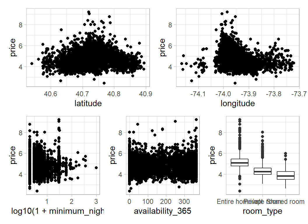
Room type is strongly predictive but the patterns in the other plots are weak.
Linear regression
To provide a baseline, I first run a linear regression
library(broom)

estimateDF %>%
  mutate( room_type = factor(room_type),
          minimum_nights = log10(1+minimum_nights)) %>%
  lm( price ~ room_type + latitude + longitude +
        minimum_nights + availability_365, data=.) -> linreg

tidy(linreg) %>% print()
## # A tibble: 7 × 5
## term estimate std.error statistic p.value
## <chr> <dbl> <dbl> <dbl> <dbl>
## 1 (Intercept) -326. 13.7 -23.9 2.75e-119
## 2 room_typePrivate room -0.791 0.0152 -52.1 0
## 3 room_typeShared room -1.19 0.0491 -24.3 1.58e-123
## 4 latitude 1.43 0.136 10.5 1.60e- 25
## 5 longitude -3.69 0.163 -22.6 5.83e-108
## 6 minimum_nights -0.191 0.0201 -9.50 3.27e- 21
## 7 availability_365 0.000728 0.0000566 12.9 2.69e- 37glance(linreg) %>% print()## # A tibble: 1 × 12
## r.squ…¹ adj.r…² sigma stati…³ p.value df logLik AIC BIC devia…⁴ df.re…⁵
## <dbl> <dbl> <dbl> <dbl> <dbl> <dbl> <dbl> <dbl> <dbl> <dbl> <int>
## 1 0.459 0.458 0.512 705. 0 6 -3748. 7513. 7565. 1311. 4993
## # … with 1 more variable: nobs <int>, and abbreviated variable names
## # ¹r.squared, ²adj.r.squared, ³statistic, ⁴deviance, ⁵df.residualThe validation RMSE for this model is
validateDF %>%
  mutate( room_type = factor(room_type),
          minimum_nights = log10(1+minimum_nights)) %>%
  mutate( mu = predict(linreg, newdata = .) ) %>%
  summarise(RMSE = sqrt( mean( (price - mu)^2)))
## # A tibble: 1 × 1
## RMSE
## <dbl>
## 1 0.492The validation RMSE is 0.492. For comparison, the leading entry on the sliced leaderboard scored 0.408 with the full test data. My earlier post used XGBoost and achieved a RMSE of 0.431, which I reduced to 0.418 with hyperparameter tuning.
BART
The BART package provides functions for fitting the BART model to different types of response. In the case of a continuous response the appropriate function is called wbart(). To run this function, the data need to be saved in vectors and matrices.
# --- Place the response and predictors in matrices -----

# --- estimation data -----------------------------------
estimateDF %>%
  pull(price) -> Y

estimateDF %>%
    mutate( room_type = as.numeric(factor(room_type)),
            minimum_nights = log10(1+minimum_nights)) %>%
    select(room_type, latitude, longitude, minimum_nights,
           availability_365) %>%
    as.matrix() -> X

# --- validation data -----------------------------------
validateDF %>%
  pull(price) -> YV

validateDF %>%
    mutate( room_type = as.numeric(factor(room_type)),
            minimum_nights = log10(1+minimum_nights)) %>%
    select(room_type, latitude, longitude, minimum_nights,
           availability_365) %>%
    as.matrix() -> XV
I start by running wbart() with default values for all of its parameters. This combines 200 trees over a chain of length 1000 following a burn-in of 100. To help assess convergence, I run three chains with different seeds. Each chain takes about 20s to run on my desktop.
My function reportBART() summarises the results of a chain. The function’s code is given in the accompanying methods post.
# --- Chain 1 -----------------------------------------
set.seed(4592)
bt1 <- wbart(x.train = X, y.train = Y, x.test = XV)
reportBART(bt1, Y, YV)
# --- Chain 2 -----------------------------------------
set.seed(2893)
bt2 <- wbart(x.train = X, y.train = Y, x.test = XV)
reportBART(bt2, Y, YV)
# --- Chain 3 -----------------------------------------
set.seed(7872)
bt3 <- wbart(x.train = X, y.train = Y, x.test = XV)
reportBART(bt3, Y, YV)
## 200 trees: run length 1000 burnin 100 thin by 1
## Posterior mean sigma 0.4498403
## Average splits per tree 1.193965
## training RMSE 0.4418989
## test RMSE 0.4539434## 200 trees: run length 1000 burnin 100 thin by 1
## Posterior mean sigma 0.4502711
## Average splits per tree 1.18779
## training RMSE 0.4418881
## test RMSE 0.4533676## 200 trees: run length 1000 burnin 100 thin by 1
## Posterior mean sigma 0.4508597
## Average splits per tree 1.17109
## training RMSE 0.442924
## test RMSE 0.4539443The validation RMSE (labelled test RMSE by my function) is 0.454, better than linear regression, but worse than my XGBoost model. In fact, 0.454 is embarrassingly good, if that performance were to carry over to the test data, it would rank 6th on the private leaderboard.
Notice that there is little evidence of over-fitting, as the training and test RMSE are similar. The summary tables also show that the trees generated by the algorithm are very stumpy, they average under 1.2 splits per tree.
Before using this model, I need to check that the algorithm has converged. I discuss convergence checking in the methods post, so here I will just present results.
Here are the trace plots for sigma, the inherent variation about the trend.
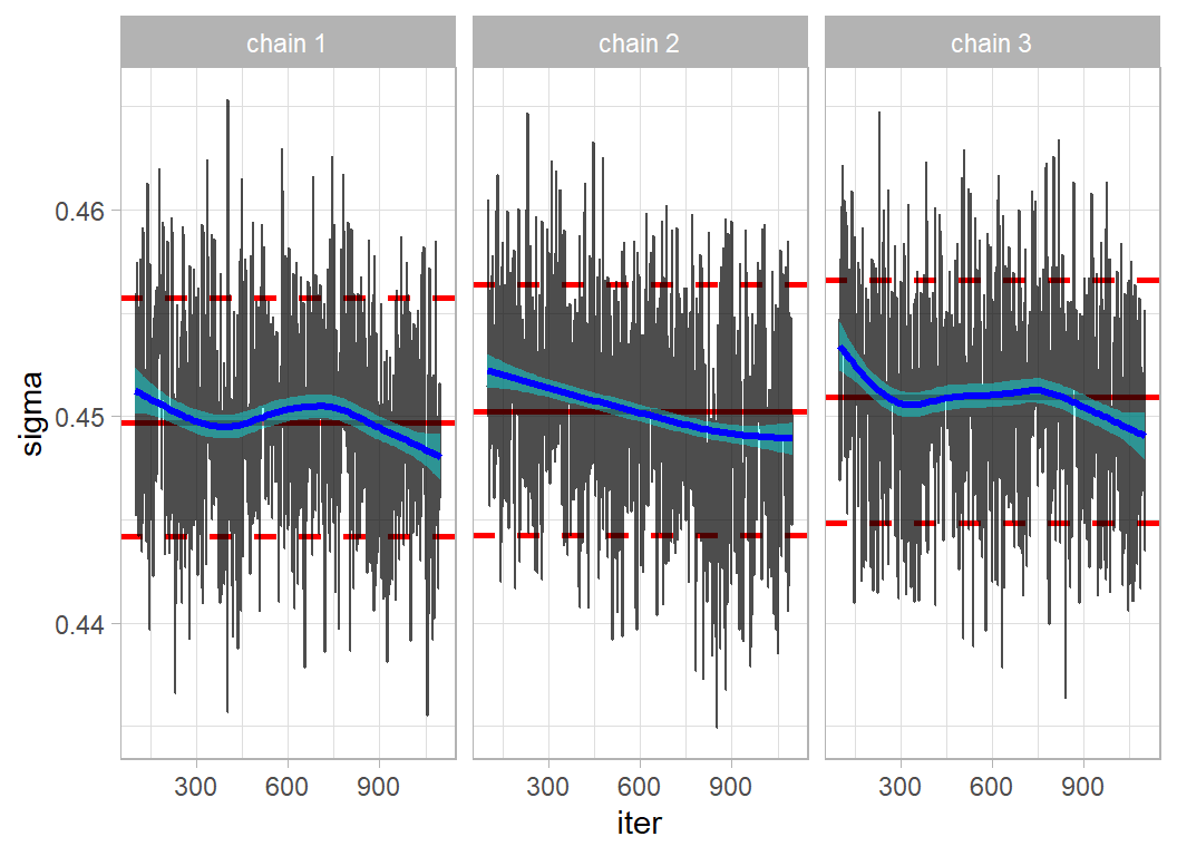
Mixing is quite good but the 3 chains are still drifting down, which suggests that I need a longer burn-in.
Here is the trace plot for 3 chains with the burn-in increased for 100 to 5000. These chains each take about 100 seconds to run.
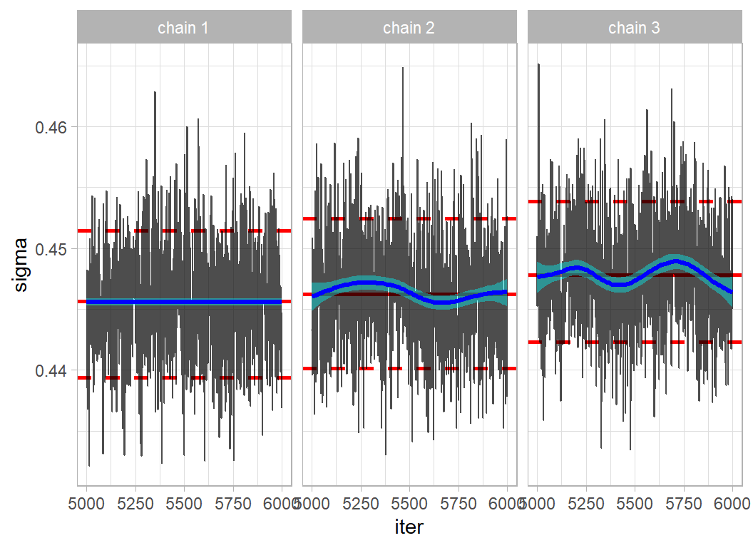
Agreement is better, but not ideal. The validation (test) RMSE has hardly changed; it is still around 0.454.
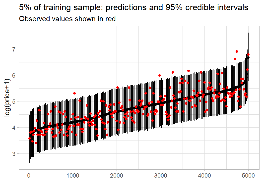
Using code developed in the methods post, I look at the in-sample predictive performance. With 5000 observations the plot is very crowded, so I only show every 20th observation.
Here is the equivalent plot for the validation sample.
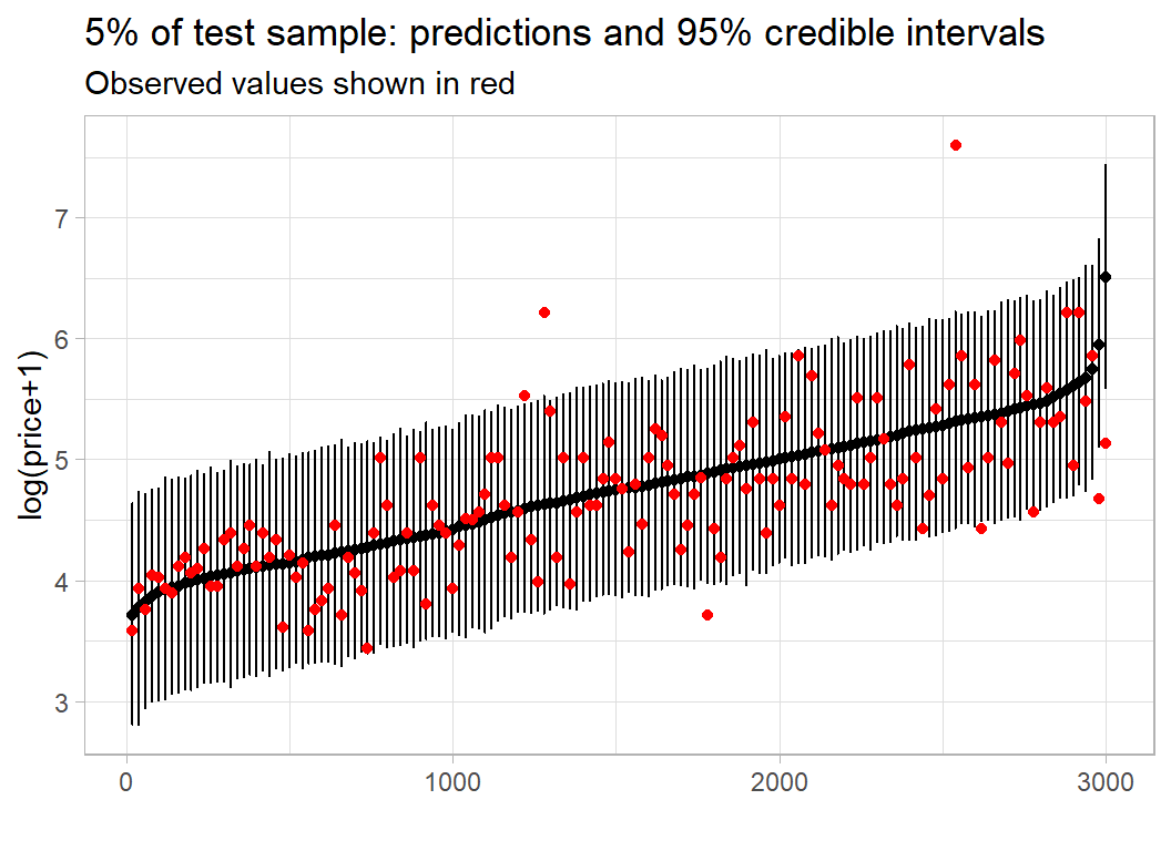
In both cases, the performance is much as expected.
wbart() returns an object that includes the number of times that each predictor is used to split a tree. This provides a measure of variable importance. The plot below shows the average usage per tree based on the first of the chains with a 5000 burn-in.
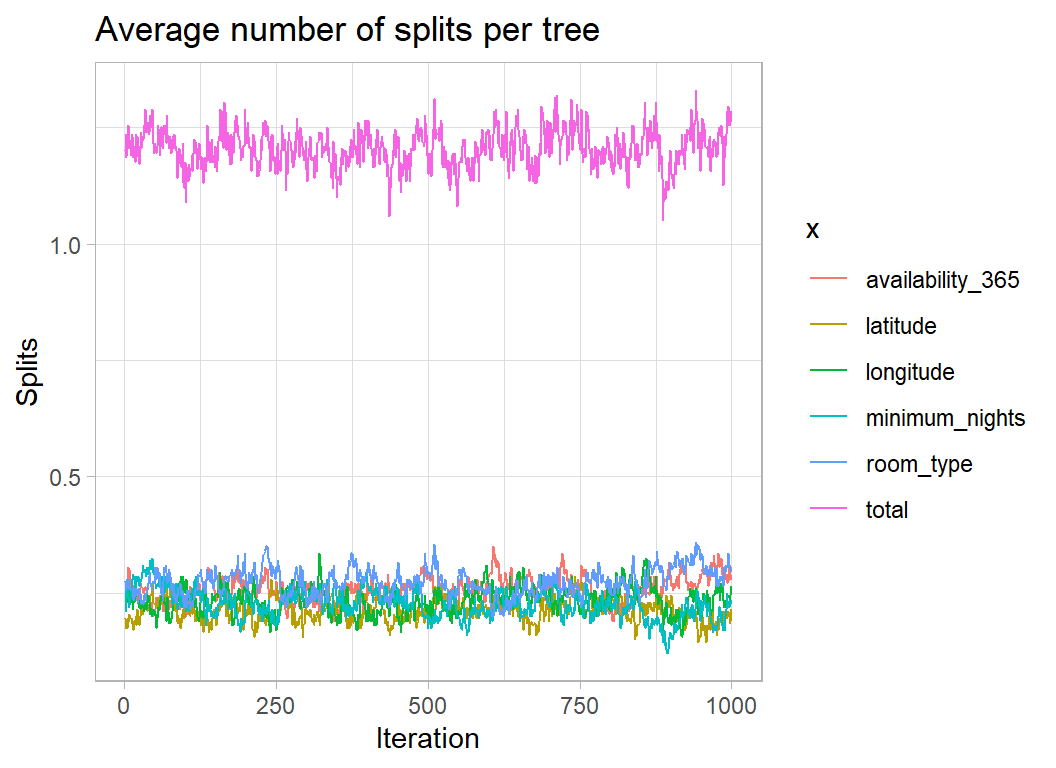
Room type is used more than the other predictors but not by as much as I would have thought. I guess that this is because there are only 3 levels of room type and once a couple of the trees have split on room type, there is nothing to be gained by reusing that predictor. This is a weakness of using the number of splits as a measure of variable importance.
The full set of predictors
In my original post on these data, I performed extensive feature selection that included identifying 134 neighbourhoods within New York and 174 key words extracted from the host’s description of the property. To these predictors, I add the number of reviews per month and the number of properties listed by the host, some hosts rent out a single property, but others rent out multiple properties and run as a business. Adding these predictors to the five used in the initial analysis gives a total of 315 potential predictors.
After redefining the matrices that contain the predictors, I re-ran the BART analysis. I found that a 5000 burn-in still produced a chain that was drifting, so I increased the burn-in to 10,000.
# --- Chain 1 -----------------------------------------
set.seed(4592)
bt1 <- wbart(x.train = X, y.train = Y, x.test = XV, nskip=10000)
reportBART(bt1, Y, YV)
# --- Chain 2 -----------------------------------------
set.seed(2893)
bt2 <- wbart(x.train = X, y.train = Y, x.test = XV, nskip=10000)
reportBART(bt2, Y, YV)
# --- Chain 3 -----------------------------------------
set.seed(7872)
bt3 <- wbart(x.train = X, y.train = Y, x.test = XV, nskip=10000)
reportBART(bt3, Y, YV)
Each chain took about 6 minutes to run.
## 200  trees: run length  1000  burnin  10000  thin by  1
##  Posterior mean sigma     0.4151023
##  Average splits per tree  1.10736
##  training RMSE            0.4055802
##  test RMSE                0.4249677
## 200 trees: run length 1000 burnin 10000 thin by 1
## Posterior mean sigma 0.4159613
## Average splits per tree 1.129745
## training RMSE 0.4058217
## test RMSE 0.4287977## 200 trees: run length 1000 burnin 10000 thin by 1
## Posterior mean sigma 0.4148526
## Average splits per tree 1.138465
## training RMSE 0.4050159
## test RMSE 0.4235205Here is the trace plot of sigma
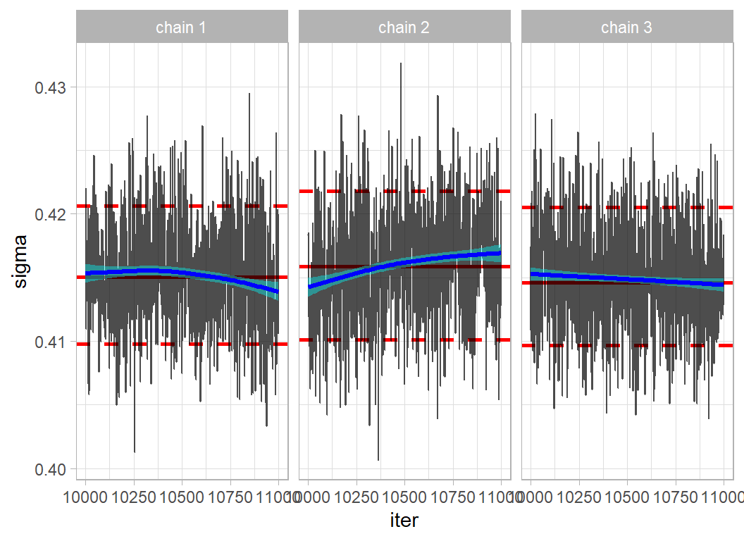
Not perfect but usable. The test RMSE is now about 0.425, better than the default XGBoost model, though that RMSE was based on the test data supplied by sliced.
Here are the average frequencies (per 200 trees) with which the main predictors were used for splitting.
# --- frequ3ncies of use in 200 trees --------------------
apply(bt1$varcount, 2, mean) %>%
  as_tibble() %>%
  mutate( var = colnames(bt1$varcount)) %>%
  rename( freq = value )  %>%
  filter( freq > 1 ) %>%
  arrange( desc(freq) ) %>%
  relocate( var, freq) %>%
  print()
## # A tibble: 57 × 2
## var freq
## <chr> <dbl>
## 1 longitude 6.63
## 2 availability_365 5.28
## 3 calculated_host_listings_count 4.43
## 4 room_type 4.30
## 5 latitude 3.71
## 6 minimum_nights 3.38
## 7 X18 2.95
## 8 N78 2.81
## 9 reviews_per_month 2.30
## 10 N120 2.21
## # … with 47 more rowsIn chain 1, 57 predictors were used more than once per set of 200 trees.
The results for the other two chains are similar, but the order of importance changes slightly. For example, here is the order for chain 3.
# --- frequencies of use in 200 trees --------------------
apply(bt3$varcount, 2, mean) %>%
  as_tibble() %>%
  mutate( var = colnames(bt1$varcount)) %>%
  rename( freq = value )  %>%
  filter( freq > 1 ) %>%
  arrange( desc(freq) ) %>%
  relocate( var, freq) %>%
  print()
## # A tibble: 57 × 2
## var freq
## <chr> <dbl>
## 1 room_type 7.13
## 2 longitude 6.44
## 3 availability_365 5.20
## 4 calculated_host_listings_count 5.08
## 5 latitude 4.43
## 6 minimum_nights 3.78
## 7 N36 2.68
## 8 N78 2.33
## 9 reviews_per_month 2.27
## 10 X18 2.21
## # … with 47 more rowsSparsity-inducing priors
So far, I have not changed any of the default priors. In my limited experience, the defaults are well-chosen and making small changes to them does not noticeably alter the fitted model.
Even changing the number of trees, only has a small impact on performance. The original papers on the BART algorithm suggested summing over 50 trees, rather than the 200 that BART defaults to. When the algorithm is limited to 50 trees, it tends to make those trees deeper, but ends with a similar predictive performance. I think that 200 trees is a marginally better choice.
One interesting choice made when setting the priors is the probability with which the predictors are chosen when the model seeks to extend a tree. The default is to make each predictor equally likely to be tried, though of course, poorly performing predictors will get rejected and will not make it into the final model.
In 2018, Antonio Linero published a paper that advocated the use of sparsity-inducing priors that encourage the model to use a smaller set of predictors.
Linero, A. R. (2018).
Bayesian regression trees for high-dimensional prediction and variable selection.
Journal of the American Statistical Association, 113(522), 626-636.
Suppose that there are J potential predictors (J=315 for my model). When the default analysis picks a predictor to add to the tree, each one has a probability 1/J of being chosen. Instead, Linero suggests making the selection probabilities follow a Dirichlet distribution with equal parameters \(\theta/J\). The model then places a beta prior on \(\theta\) and treats the selection probabilities of the predictors as parameters to be learnt.
The form of the prior on \(\theta\) is, \[ \frac{\theta}{\theta+\rho} \sim \text{Beta}(a, b) \] where the user chooses a, b and \(\rho\). The defaults are a=0.5, b=1, \(\rho\)=J.
Although, the Dirichlet prior starts by treating all predictors equally, the model is free to learn which predictors are most useful and to use that information when selecting a new predictor to use in the BART model. By changing, a, b and \(\rho\), the user changes the sparsity of the selection. Once BART has identified the important predictors, it tends to stick with them.
I tried changing a and b but found that they have little impact on the airbnb model. However, reducing \(\rho\) does make the predictor selection more sparse. Below, I show the results for \(\rho\)=100.
# --- single sparse chain -----------------------------
set.seed(4592)
bt1 <- wbart(x.train = X, y.train = Y, x.test = XV,
             nskip=10000, sparse=TRUE, rho=100)
reportBART(bt1, Y, YV)
## 200 trees: run length 1000 burnin 10000 thin by 1
## Posterior mean sigma 0.408865
## Average splits per tree 1.28454
## training RMSE 0.3983437
## test RMSE 0.4229048The chain took about 3.5 minutes to run.
The tree depths have increased very slightly and the test RMSE is slightly better. Remember that a default XGBoost model had a RMSE of 0.431 (though that was with the sliced test data).
Here are the frequencies for the top predictors
## # A tibble: 39 × 2
##    var                             freq
##    <chr>                          <dbl>
##  1 calculated_host_listings_count 37.6
##  2 room_type                      36.2
##  3 longitude                      21.4
##  4 availability_365               19.4
##  5 N78                            16.9
##  6 latitude                        9.49
##  7 X11                             6.30
##  8 X18                             5.95
##  9 X3                              5.71
## 10 minimum_nights                  5.36
## # … with 29 more rows
Notice that the frequencies have increased dramatically, so that fewer predictors are used.
Finally, here are the selection probabilities that the model learns from its Dirichlet prior. The order is more or less the same as that for the frequencies.
## # A tibble: 21 × 2
##    var                              prob
##    <chr>                           <dbl>
##  1 calculated_host_listings_count 0.135
##  2 room_type                      0.130
##  3 longitude                      0.0772
##  4 availability_365               0.0697
##  5 N78                            0.0606
##  6 latitude                       0.0349
##  7 X11                            0.0228
##  8 X18                            0.0212
##  9 X3                             0.0207
## 10 minimum_nights                 0.0197
## # … with 11 more rows
Conclusions
I was struck by the speed of the BART algorithm, unlike many Bayesian models, it really is a practical option for moderate sized problems.
The default priors are well-chosen, but even saying that is to deny the Bayesian method. A true Bayesian would want to select the priors based on their genuine beliefs, To say that the priors are well-chosen, just means that they give good predictions for a wide range of problems. Do the default values of power and base really reflect a belief about how deep the trees should be? I have my doubts. It may just be a reflection of my purist tendencies, but “it works” is not enough for me.