Sliced Episode 10: Animal adoption
Introduction
The data for episode 10 of Sliced, the second round of the play-offs, relates to the adoption of abandoned or unwanted pets. Given information about the animal, such as its breed and age, the competitors had to predict a three class outcome, either, adoption, transfer or what is euphemistically called ‘no outcome’, which in reality means that the animal was put down (another euphemism).
The data can be downloaded from https://www.kaggle.com/c/sliced-s01e10-playoffs-2/overview/description.
In truth this is not a particularly interesting dataset. There are few features and apart from the three class outcome, it is a very standard problem.
In an attempt to make it more interesting, I decided to experiment with the mlr3 package. This is a competitor to tidymodels in the sense that it offers another way of organising machine learning workflows. I do not like tidymodels because I feel that it encourages a black box mentality, so I was interested to see if I have the same reaction to mlr3.
In this post, I will concentrate of the application of mlr3 to the animal adoption data without giving a detailed explanation of the syntax. If you have never seen mlr3 before, you might find it helpful to start by reading my methods post entitled Methods: Introduction to mlr3. In that post I explain how the structure of mlr3 is dependent on object orientated programming and in particular, the R6 package.
Reading the data:
It is my practice to read the data asis and to immediately save it in rds format within a directory called data/rData. For details of the way that I organise my analyses you should read my post called Sliced Methods Overview.
# --- setup: libraries & options ------------------------
library(tidyverse)

theme_set( theme_light())

# --- set home directory -------------------------------
home <- "C:/Projects/kaggle/sliced/s01-e10"

# --- read downloaded data -----------------------------
trainRawDF <- readRDS( file.path(home, "data/rData/train.rds") )

testRawDF <- readRDS( file.path(home, "data/rData/test.rds") )
Data Exploration:
I usually start by summarising the training data with the skimr package.
# --- summarise the training set -----------------------
skimr::skim(trainRawDF)
I’ve hidden the output but in brief it shows that there are 54,408 animals in the training data and their outcomes cover the period 7th Nov 2015 to 1 Feb 2018. There are only a few missing values, except for the animal’s name, which is missing for about 30% of the animals.
Response
The majority of the animals are adopted
# --- outcomes ----------------------------------------
trainRawDF %>%
  count( outcome_type ) %>%
  mutate( pct = 100*n/sum(n))
## # A tibble: 3 x 3
## outcome_type n pct
## <chr> <int> <dbl>
## 1 adoption 33275 61.2
## 2 no outcome 4735 8.70
## 3 transfer 16398 30.1Predictors
As I have often done in previous episodes of Spliced, I have written a function for plotting the predictors; this time the function is called plot_animals(). The code is given in as a appendix at the end of this post.
Here is the pattern of outcomes for the 4 major animal types.
# --- categories of animal type ---------------------------
trainRawDF %>%
  plot_animals(animal_type)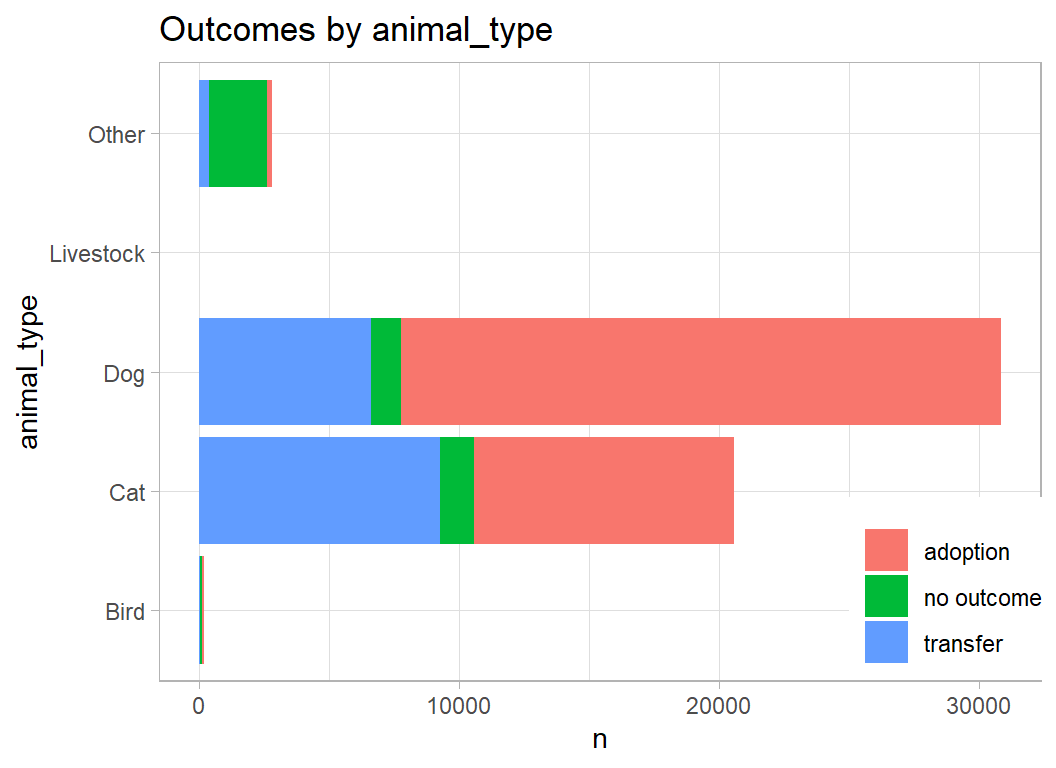
Two thoughts come to mind.
- the features relevant to prediction for cats, dogs and birds will be very different
- the bird & livestock categories are very small
I will split the data into three parts; cat, dog & (other+bird+livestock) and I will predict separately within each of the three.
Data cleaning
In preparation for the analysis, I need to process the date on which the outcome occurred, which I’ll convert to a month and a year, and I need to clean the ages, which are variously recorded in days or months or years. I will not use the data_of_birth.
There are a handful of missing ages that I replace using the median age for that type of animal.
# --- clean the training data --------------------------------
library(lubridate)

trainRawDF %>%
   mutate( outcome_type = factor(outcome_type),
           # --- date to month, year and time of day ---------
           month         = as.numeric(month(datetime)),
           year          = as.numeric(year(datetime)),
           hour          = as.numeric(hour(datetime)),
           # --- numerical part of the age field -------------
           age_number    = as.numeric(str_extract(
             age_upon_outcome, "[:digit:]+")),
           # --- test part of the age field ------------------
           age_unit      = str_extract(
             age_upon_outcome, "[a-z]+"),
           unit          = substr(age_unit, 1, 1)) %>%
  # --- calculate age in years -------------------------------
  mutate(   age = age_number*(unit == "y") +
                  age_number*(unit == "m")/12 +
                  age_number*(unit == "w")/52 +
                  age_number*(unit == "d")/365 ) %>%
  select(-age_upon_outcome, -age_number, -age_unit, -unit,
         -datetime, -date_of_birth, -name) -> prepDF

# median impute the missing ages ------------------------------
# --- median = 2 for dogs -------------------------------------
mDog <- median(prepDF$age[prepDF$animal_type=="Dog"], na.rm=TRUE)

prepDF$age[is.na(prepDF$age) & prepDF$animal_type=="Dog"] <- mDog

# --- median = 1 for bats -------------------------------------
mBat <- median(prepDF$age[prepDF$breed=="Bat Mix"], na.rm=TRUE)

prepDF$age[is.na(prepDF$age) & prepDF$breed=="Bat Mix"] <- mBat
Cats
Skimming the data on cats shows that there are 20,561 rows, 70 breeds and 201 colours.
skimr::skim(prepDF %>% filter(animal_type == "Cat"))Here are the common cat breeds
# --- categories of cat breed ---------------------------
prepDF %>%
  filter( animal_type == "Cat") %>%
  mutate( breed = fct_lump(breed, prop=0.005)) %>%
  plot_animals(breed)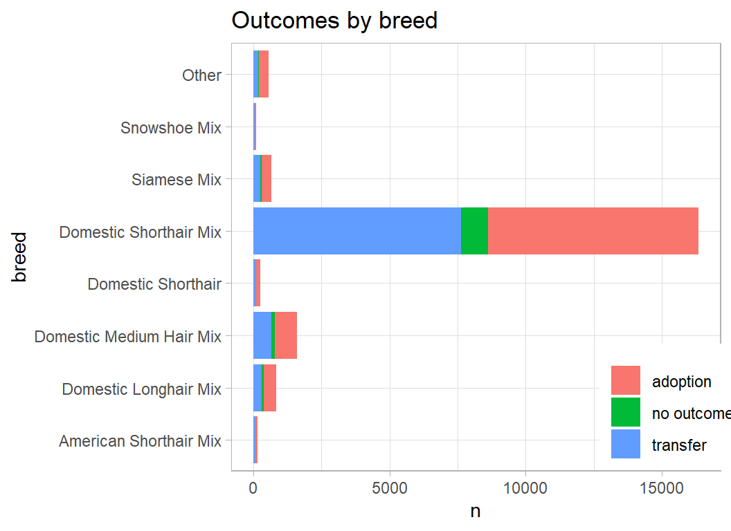
The common colours are not obviously related to outcome.
# --- categories of cat breed ---------------------------
prepDF %>%
  filter( animal_type == "Cat") %>%
  mutate( colour = fct_lump(color, prop=0.01)) %>%
  plot_animals(colour)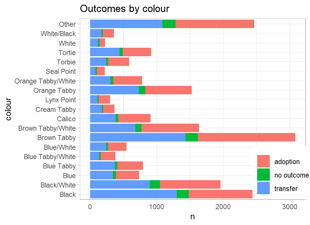
Neutered cats are more likely to get adopted
# --- neutering in cats ---------------------------------
prepDF %>%
  filter( animal_type == "Cat") %>%
  plot_animals(spay_neuter)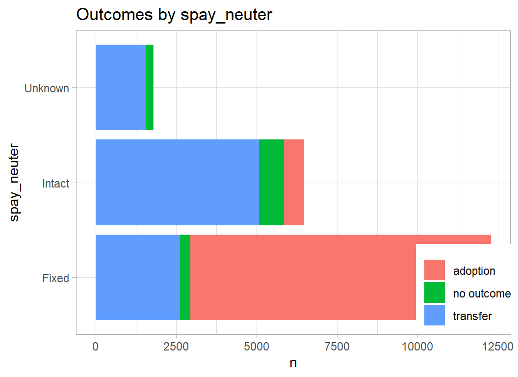
The cat’s sex is not particularly predictive, but when the sex is unknown it is unlikely that the cat was adopted.
prepDF %>%
  filter( animal_type == "Cat") %>%
  plot_animals(sex)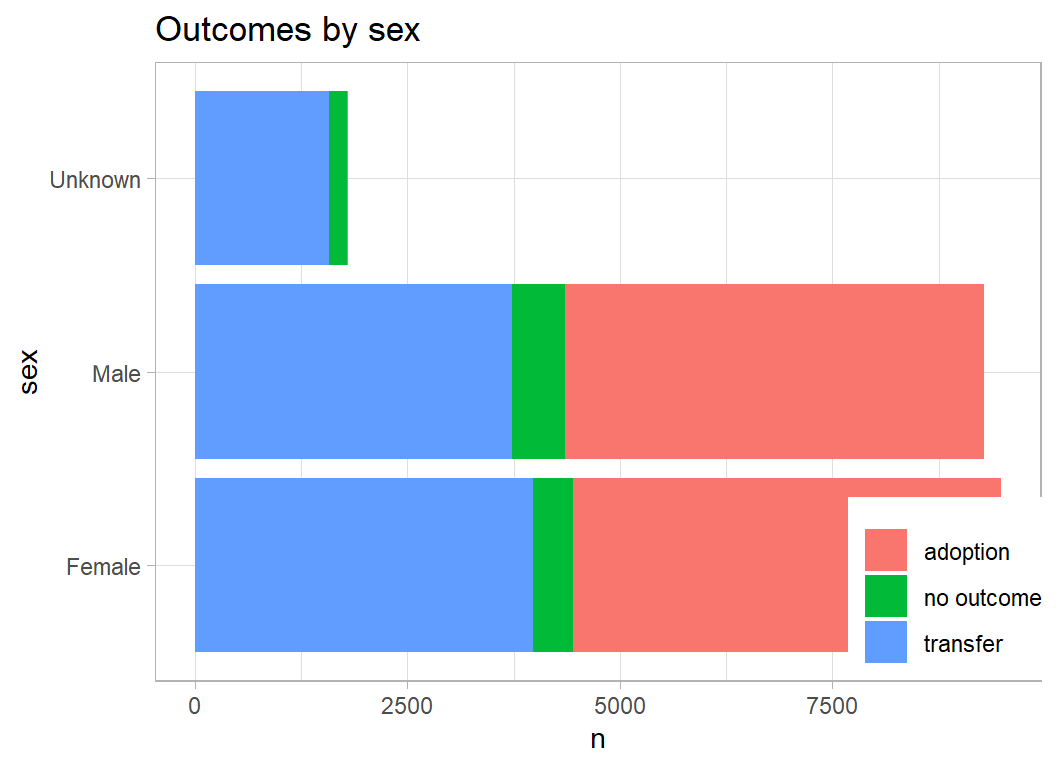
Age is recorded is days, weeks, months or years but has been records as fractions of a year.
prepDF %>%
  filter( animal_type == "Cat") %>%
  mutate( ageGp = cut(age, breaks=c(0, 1, 2, 15))) %>%
  plot_animals(ageGp)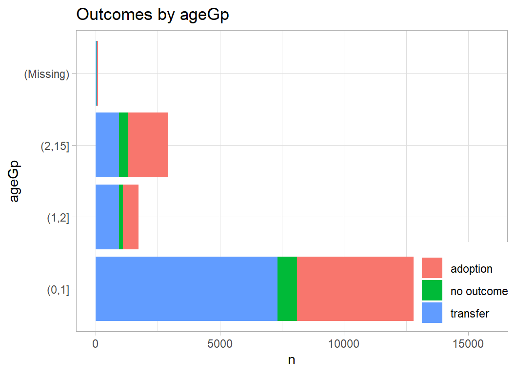
The outcomes vary considerably across the year with a larger proportion of transfers in April and May.
prepDF %>%
  filter( animal_type == "Cat") %>%
  mutate( month = factor(month, levels=1:12, labels=month.abb)) %>%
  plot_animals(month)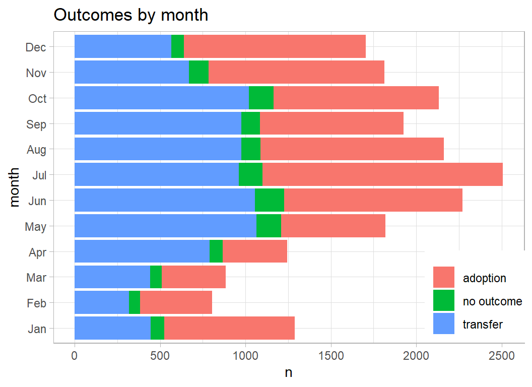
Transfers are less common in recent years
prepDF %>%
  filter( animal_type == "Cat") %>%
  mutate( year = factor(year)) %>%
  plot_animals(year)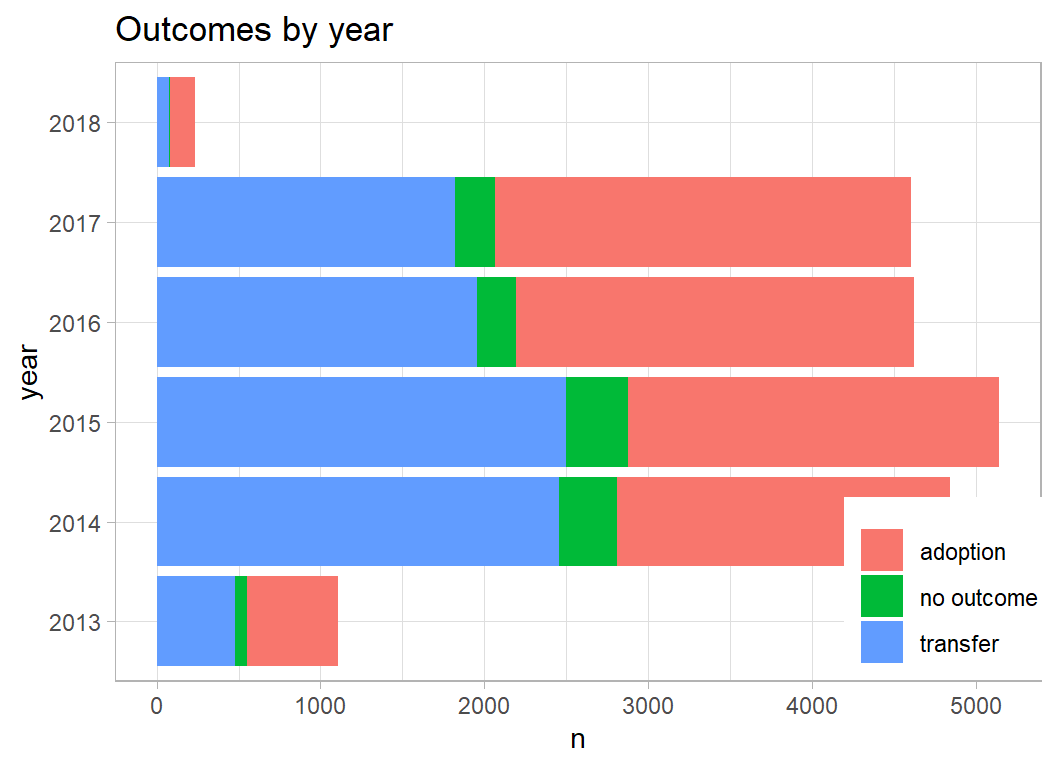
It seems like cheating, but work patterns clearly help predict outcome. Transfers occur at 9am, but people call after work to collect their adopted cat.
prepDF %>%
  filter( animal_type == "Cat") %>%
  mutate( hour = factor(hour)) %>%
  plot_animals(hour)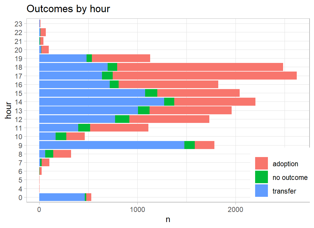
Preprocessing cats
I’ll add some indicator variables for the common colours and breeds and prepare a data set for training the cat model.
# --- function to add indicators ----------------------------
add_indicators <- function(thisDF, col, keywords, prefix) {
  for( j in seq_along(keywords) ) {
     thisDF[[ paste(prefix, j, sep="")]] <-
       as.numeric( str_detect(tolower(thisDF[[col]]), keywords[j]))
  }
  return(thisDF)
}
# --- select the cats ---------------------------------------
prepDF %>%
  filter(animal_type == "Cat") %>%
  select( -animal_type ) -> prepCatDF

# --- indicators for key words in breed ---------------------
add_indicators(prepCatDF,
               col = "breed",
               keywords = c("domestic", "mix", "short",
                           "medium", "long"),
               prefix = "B") -> prepCatDF

# --- indicators for key words in colour ---------------------
add_indicators(prepCatDF,
               col = "color",
               keywords = c("tabby", "black", "white",
                            "brown", "blue"),
               prefix = "C") -> prepCatDF

# --- indicators for sex -------------------------------------
add_indicators(prepCatDF,
               col = "sex",
               keywords = sort(unique(tolower(prepCatDF$sex))),
               prefix = "S") -> prepCatDF

# --- indicators for neuter ---------------------------------
add_indicators(prepCatDF,
               col = "spay_neuter",
               keywords = sort(unique(tolower(prepCatDF$spay_neuter))),
               prefix = "N") -> prepCatDF

# --- keep predictors ---------------------------------------
prepCatDF %>%
  select( -breed, -color, -sex, -spay_neuter,  -id) -> trainCatDF
mlr3
Now I will use mlr3 to model the cat data. For an explanation of how mlr3 works, you should read my post entitled Methods: Introduction to mlr3. Briefly, the terminology is
* task … the data
* learner … the method of model building
* measure … the performance metric
Rather like loading the tidyverse, loading mlr3verse makes available all of the essential packages in the ecosystem.
I want to do something simple, so that I do not have to explain the method at the same time as introducing mlr3, so I’ll use xgboost
In the following code, I define the data, select a learner, train the model, look at the results, makes predictions and inspect the confusion matrix; I end by choosing the logloss as my performance metric and I evaluate the logloss on the training data.
Once you understand the syntax, the code is concise and logical.
# --- load the important mlr3 packages -----------------------
library(mlr3verse)

# --- define the task ----------------------------------------
myTask <- TaskClassif$new( id      = "cat_adoption",
                           backend = trainCatDF,
                           target  = "outcome_type")

# --- select the learner -------------------------------------
myLearner <- lrn("classif.xgboost",
                 nrounds     = 100,
                 objective   = "multi:softprob",
                 eval_metric = "mlogloss")

# --- train the model ----------------------------------------
myLearner$train(task = myTask)

# --- look at the result -------------------------------------
myLearner$model
## ##### xgb.Booster
## raw: 967.8 Kb
## call:
## xgboost::xgb.train(data = data, nrounds = 100L, watchlist = list(
## train = <pointer: 0x0000000018664570>), verbose = 0L, nthread = 1L,
## objective = "multi:softprob", eval_metric = "mlogloss", num_class = 3L)
## params (as set within xgb.train):
## nthread = "1", objective = "multi:softprob", eval_metric = "mlogloss", num_class = "3", validate_parameters = "TRUE"
## xgb.attributes:
## niter
## callbacks:
## cb.evaluation.log()
## # of features: 20
## niter: 100
## nfeatures : 20
## evaluation_log:
## iter train_mlogloss
## 1 0.862690
## 2 0.727069
## ---
## 99 0.301958
## 100 0.300915# --- predict and show the confusion matrix ------------------
myPredictions <- myLearner$predict(myTask)
myPredictions$confusion## truth
## response adoption no outcome transfer
## adoption 9370 166 1119
## no outcome 13 630 37
## transfer 593 505 8128# --- logloss requires probability predictions ---------------
myMeasure <- msr("classif.logloss")
myLearner$predict_type <- "prob"
myPredictions <- myLearner$predict(myTask)
myPredictions$score(myMeasure)## classif.logloss
## 0.3009133The in-sample logloss is 0.30. It only relates to cats, but for comparison, the leading model in the competition scored a test sample logloss of 0.36 over all animals.
I can access the results in the normal way since myLearner$model contains the usual structure returned by xgboost.
myLearner$model$evaluation_log %>%
    ggplot( aes(x=iter, y=train_mlogloss)) +
    geom_line(colour="blue") +
    scale_y_continuous( limits = c(0, 1), breaks=seq(0, 1, by=.05)) +
    labs(x="Iteration", y="mean log loss",
         title="In-sample multiclass log loss")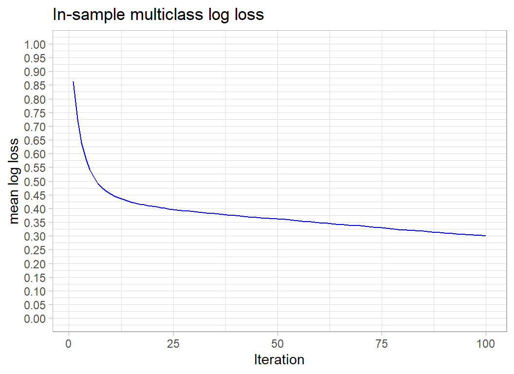
I need to check if the in-sample logloss has overfitted, so I’ll use cross-validation with 5 folds and I’ll speed things up by running the folds in multiple sessions using the future package. When you use multiple sessions each one runs independently and has its own copy of the data. mlr3 also allows multiple cores, when the cores access the same data, but this is not available in Windows.
future::plan("multisession")

# --- define CV and apply to the data -----------------------
set.seed(9766)
myCV <- rsmp("cv", folds=5)
myCV$instantiate(task = myTask)

# --- run the cross validation ------------------------------
rsFit <- resample( task       = myTask,
                   learner    = myLearner,
                   resampling = myCV)
## INFO [15:33:54.386] [mlr3] Applying learner 'classif.xgboost' on task 'cat_adoption' (iter 5/5)
## INFO [15:33:55.715] [mlr3] Applying learner 'classif.xgboost' on task 'cat_adoption' (iter 2/5)
## INFO [15:33:57.044] [mlr3] Applying learner 'classif.xgboost' on task 'cat_adoption' (iter 4/5)
## INFO [15:33:58.735] [mlr3] Applying learner 'classif.xgboost' on task 'cat_adoption' (iter 3/5)
## INFO [15:34:00.383] [mlr3] Applying learner 'classif.xgboost' on task 'cat_adoption' (iter 1/5)# --- show individual and aggregate logloss -----------------
rsFit$score(myMeasure)## task task_id learner learner_id
## 1: <TaskClassif[47]> cat_adoption <LearnerClassifXgboost[35]> classif.xgboost
## 2: <TaskClassif[47]> cat_adoption <LearnerClassifXgboost[35]> classif.xgboost
## 3: <TaskClassif[47]> cat_adoption <LearnerClassifXgboost[35]> classif.xgboost
## 4: <TaskClassif[47]> cat_adoption <LearnerClassifXgboost[35]> classif.xgboost
## 5: <TaskClassif[47]> cat_adoption <LearnerClassifXgboost[35]> classif.xgboost
## resampling resampling_id iteration prediction
## 1: <ResamplingCV[19]> cv 1 <PredictionClassif[19]>
## 2: <ResamplingCV[19]> cv 2 <PredictionClassif[19]>
## 3: <ResamplingCV[19]> cv 3 <PredictionClassif[19]>
## 4: <ResamplingCV[19]> cv 4 <PredictionClassif[19]>
## 5: <ResamplingCV[19]> cv 5 <PredictionClassif[19]>
## classif.logloss
## 1: 0.4467382
## 2: 0.4358017
## 3: 0.4627691
## 4: 0.4434847
## 5: 0.4586902rsFit$aggregate(myMeasure)## classif.logloss
## 0.4494968The cross-validated logloss is 0.45, so the in-sample result was very optimistic and the model is actually quite some way from the top of the leaderboard.
I will try some classic machine learning hyperparameter tuning, even though I don’t really approve, because it serves to demonstrate more features of mlr3. myLearner$param_set contains the values of the parameters that were used to fit the model.
myLearner$param_set ## <ParamSet>
## id class lower upper nlevels default
## 1: alpha ParamDbl 0 Inf Inf 0
## 2: approxcontrib ParamLgl NA NA 2 FALSE
## 3: base_score ParamDbl -Inf Inf Inf 0.5
## 4: booster ParamFct NA NA 3 gbtree
## 5: callbacks ParamUty NA NA Inf <list[0]>
## 6: colsample_bylevel ParamDbl 0 1 Inf 1
## 7: colsample_bynode ParamDbl 0 1 Inf 1
## 8: colsample_bytree ParamDbl 0 1 Inf 1
## 9: early_stopping_rounds ParamInt 1 Inf Inf
## 10: eta ParamDbl 0 1 Inf 0.3
## 11: eval_metric ParamUty NA NA Inf error
## 12: feature_selector ParamFct NA NA 5 cyclic
## 13: feval ParamUty NA NA Inf
## 14: gamma ParamDbl 0 Inf Inf 0
## 15: grow_policy ParamFct NA NA 2 depthwise
## 16: interaction_constraints ParamUty NA NA Inf <NoDefault[3]>
## 17: lambda ParamDbl 0 Inf Inf 1
## 18: lambda_bias ParamDbl 0 Inf Inf 0
## 19: max_bin ParamInt 2 Inf Inf 256
## 20: max_delta_step ParamDbl 0 Inf Inf 0
## 21: max_depth ParamInt 0 Inf Inf 6
## 22: max_leaves ParamInt 0 Inf Inf 0
## 23: maximize ParamLgl NA NA 2
## 24: min_child_weight ParamDbl 0 Inf Inf 1
## 25: missing ParamDbl -Inf Inf Inf NA
## 26: monotone_constraints ParamUty NA NA Inf 0
## 27: normalize_type ParamFct NA NA 2 tree
## 28: nrounds ParamInt 1 Inf Inf 1
## 29: nthread ParamInt 1 Inf Inf 1
## 30: ntreelimit ParamInt 1 Inf Inf
## 31: num_parallel_tree ParamInt 1 Inf Inf 1
## 32: objective ParamUty NA NA Inf binary:logistic
## 33: one_drop ParamLgl NA NA 2 FALSE
## 34: outputmargin ParamLgl NA NA 2 FALSE
## 35: predcontrib ParamLgl NA NA 2 FALSE
## 36: predictor ParamFct NA NA 2 cpu_predictor
## 37: predinteraction ParamLgl NA NA 2 FALSE
## 38: predleaf ParamLgl NA NA 2 FALSE
## 39: print_every_n ParamInt 1 Inf Inf 1
## 40: rate_drop ParamDbl 0 1 Inf 0
## 41: refresh_leaf ParamLgl NA NA 2 TRUE
## 42: reshape ParamLgl NA NA 2 FALSE
## 43: sample_type ParamFct NA NA 2 uniform
## 44: save_name ParamUty NA NA Inf
## 45: save_period ParamInt 0 Inf Inf
## 46: scale_pos_weight ParamDbl -Inf Inf Inf 1
## 47: sketch_eps ParamDbl 0 1 Inf 0.03
## 48: skip_drop ParamDbl 0 1 Inf 0
## 49: subsample ParamDbl 0 1 Inf 1
## 50: top_k ParamInt 0 Inf Inf 0
## 51: training ParamLgl NA NA 2 FALSE
## 52: tree_method ParamFct NA NA 5 auto
## 53: tweedie_variance_power ParamDbl 1 2 Inf 1.5
## 54: updater ParamUty NA NA Inf <NoDefault[3]>
## 55: verbose ParamInt 0 2 3 1
## 56: watchlist ParamUty NA NA Inf
## 57: xgb_model ParamUty NA NA Inf
## id class lower upper nlevels default
## parents value
## 1:
## 2:
## 3:
## 4:
## 5:
## 6:
## 7:
## 8:
## 9:
## 10:
## 11: mlogloss
## 12: booster
## 13:
## 14:
## 15: tree_method
## 16:
## 17:
## 18:
## 19: tree_method
## 20:
## 21:
## 22: grow_policy
## 23:
## 24:
## 25:
## 26:
## 27: booster
## 28: 100
## 29: 1
## 30:
## 31:
## 32: multi:softprob
## 33: booster
## 34:
## 35:
## 36:
## 37:
## 38:
## 39: verbose
## 40: booster
## 41:
## 42:
## 43: booster
## 44:
## 45:
## 46:
## 47: tree_method
## 48: booster
## 49:
## 50: booster,feature_selector
## 51:
## 52: booster
## 53: objective
## 54:
## 55: 0
## 56:
## 57:
## parents valueI will reduce the learning rate from 0.3 to 0.1 and simultaneously try tuning the number of iterations (rounds) and the max_depth parameter. The method that I’ve chosen takes 10 random pairs of parameter values within my specified ranges.
myLearner$predict_type <- "prob"

# --- set hyperparameters -----------------------------------
myLearner$param_set$values           <- list(eta=0.1)
myLearner$param_set$values$nrounds   <- to_tune(50, 500)
myLearner$param_set$values$max_depth <- to_tune(3, 6)

# --- run tuning --------------------------------------------
set.seed(9830)

myTuner <-  tune(
  method     = "random_search",
  task       = myTask,
  learner    = myLearner,
  resampling = myCV,
  measure    = myMeasure,
  term_evals = 10,
  batch_size = 5
)
I’ve suppressed the output for each iteration as it is long and boring, but here is the final result.
# --- inspect result ----------------------------------------
myTuner
## <TuningInstanceSingleCrit>
## * State: Optimized
## * Objective: <ObjectiveTuning:classif.xgboost_on_cat_adoption>
## * Search Space:
## <ParamSet>
## id class lower upper nlevels default value
## 1: nrounds ParamInt 50 500 451 <NoDefault[3]>
## 2: max_depth ParamInt 3 6 4 <NoDefault[3]>
## * Terminator: <TerminatorEvals>
## * Terminated: TRUE
## * Result:
## nrounds max_depth learner_param_vals x_domain classif.logloss
## 1: 361 5 <list[3]> <list[2]> 0.4466408
## * Archive:
## <ArchiveTuning>
## nrounds max_depth classif.logloss timestamp batch_nr
## 1: 426 4 0.45 2021-11-02 15:35:03 1
## 2: 97 4 0.46 2021-11-02 15:35:03 1
## 3: 90 5 0.45 2021-11-02 15:35:03 1
## 4: 216 3 0.45 2021-11-02 15:35:03 1
## 5: 349 6 0.45 2021-11-02 15:35:03 1
## 6: 304 6 0.45 2021-11-02 15:36:14 2
## 7: 171 3 0.46 2021-11-02 15:36:14 2
## 8: 467 5 0.45 2021-11-02 15:36:14 2
## 9: 361 5 0.45 2021-11-02 15:36:14 2
## 10: 61 3 0.48 2021-11-02 15:36:14 2The best of these random combinations has a cross-validated logloss of 0.447, slightly worse than the default model. The other point to note is that changing these hyperparameters makes little difference. I’ll stick with the defaults.
Dogs
I explored and preprocessed the dogs with very similar code to that used for cats so I have hidden the output. I ended with a dataset called trainDogDF.
Now I will run an analysis that mirrors that for cats
# --- define the task ----------------------------------------
myTask <- TaskClassif$new( id = "dog_adoption",
                 backend = trainDogDF,
                 target  = "outcome_type")

# --- select the learner -------------------------------------
myLearner <- lrn("classif.xgboost", nrounds = 100,
                 objective="multi:softprob",
                 eval_metric="mlogloss")

# --- train the model ----------------------------------------
myLearner$train(task = myTask)

# --- look at the result -------------------------------------
myLearner$model
## ##### xgb.Booster
## raw: 956.8 Kb
## call:
## xgboost::xgb.train(data = data, nrounds = 100L, watchlist = list(
## train = <pointer: 0x0000000018664930>), verbose = 0L, nthread = 1L,
## objective = "multi:softprob", eval_metric = "mlogloss", num_class = 3L)
## params (as set within xgb.train):
## nthread = "1", objective = "multi:softprob", eval_metric = "mlogloss", num_class = "3", validate_parameters = "TRUE"
## xgb.attributes:
## niter
## callbacks:
## cb.evaluation.log()
## # of features: 21
## niter: 100
## nfeatures : 21
## evaluation_log:
## iter train_mlogloss
## 1 0.877068
## 2 0.749589
## ---
## 99 0.400619
## 100 0.400271# --- predict and show the confusion matrix ------------------
myPredictions <- myLearner$predict(myTask)
myPredictions$confusion## truth
## response adoption no outcome transfer
## adoption 22503 588 3634
## no outcome 48 408 26
## transfer 494 147 2982# --- logloss requires probability predictions ---------------
myMeasure <- msr("classif.logloss")
myLearner$predict_type <- "prob"
myPredictions <- myLearner$predict(myTask)
myPredictions$score(myMeasure)## classif.logloss
## 0.4002699# --- define CV and apply to the data -----------------------
set.seed(9126)
myCV <- rsmp("cv", folds=5)
myCV$instantiate(task = myTask)
# --- run the cross validation ------------------------------
rsFit <- resample( task = myTask,
learner = myLearner,
resampling = myCV)## INFO [15:36:25.044] [mlr3] Applying learner 'classif.xgboost' on task 'dog_adoption' (iter 1/5)
## INFO [15:36:25.083] [mlr3] Applying learner 'classif.xgboost' on task 'dog_adoption' (iter 3/5)
## INFO [15:36:25.124] [mlr3] Applying learner 'classif.xgboost' on task 'dog_adoption' (iter 5/5)
## INFO [15:36:25.481] [mlr3] Applying learner 'classif.xgboost' on task 'dog_adoption' (iter 4/5)
## INFO [15:36:25.524] [mlr3] Applying learner 'classif.xgboost' on task 'dog_adoption' (iter 2/5)# --- show individual and aggregate logloss -----------------
rsFit$score(myMeasure)## task task_id learner learner_id
## 1: <TaskClassif[47]> dog_adoption <LearnerClassifXgboost[35]> classif.xgboost
## 2: <TaskClassif[47]> dog_adoption <LearnerClassifXgboost[35]> classif.xgboost
## 3: <TaskClassif[47]> dog_adoption <LearnerClassifXgboost[35]> classif.xgboost
## 4: <TaskClassif[47]> dog_adoption <LearnerClassifXgboost[35]> classif.xgboost
## 5: <TaskClassif[47]> dog_adoption <LearnerClassifXgboost[35]> classif.xgboost
## resampling resampling_id iteration prediction
## 1: <ResamplingCV[19]> cv 1 <PredictionClassif[19]>
## 2: <ResamplingCV[19]> cv 2 <PredictionClassif[19]>
## 3: <ResamplingCV[19]> cv 3 <PredictionClassif[19]>
## 4: <ResamplingCV[19]> cv 4 <PredictionClassif[19]>
## 5: <ResamplingCV[19]> cv 5 <PredictionClassif[19]>
## classif.logloss
## 1: 0.5142654
## 2: 0.5061514
## 3: 0.5052791
## 4: 0.5274591
## 5: 0.5069654rsFit$aggregate(myMeasure)## classif.logloss
## 0.5120241An in-sample logloss of 0.40 and a cross-validated logloss of 0.51. Slightly worse than the result for cats.
I’ll not bother with hyperparameter tuning but move on to the remaining animals, i.e. everything that is not a cat or a dog. I called the data frame trainRestDF.
# --- define the task ----------------------------------------
myTask <- TaskClassif$new( id = "remainder_adoption",
                 backend = trainRestDF,
                 target  = "outcome_type")

# --- select the learner -------------------------------------
myLearner <- lrn("classif.xgboost", nrounds = 100,
                 objective="multi:softprob",
                 eval_metric="mlogloss")

# --- train the model ----------------------------------------
myLearner$train(task = myTask)

# --- look at the result -------------------------------------
myLearner$model
## ##### xgb.Booster
## raw: 541.4 Kb
## call:
## xgboost::xgb.train(data = data, nrounds = 100L, watchlist = list(
## train = <pointer: 0x0000000018665530>), verbose = 0L, nthread = 1L,
## objective = "multi:softprob", eval_metric = "mlogloss", num_class = 3L)
## params (as set within xgb.train):
## nthread = "1", objective = "multi:softprob", eval_metric = "mlogloss", num_class = "3", validate_parameters = "TRUE"
## xgb.attributes:
## niter
## callbacks:
## cb.evaluation.log()
## # of features: 21
## niter: 100
## nfeatures : 21
## evaluation_log:
## iter train_mlogloss
## 1 0.787281
## 2 0.608884
## ---
## 99 0.030240
## 100 0.029763# --- predict and show the confusion matrix ------------------
myPredictions <- myLearner$predict(myTask)
myPredictions$confusion## truth
## response adoption no outcome transfer
## adoption 254 1 0
## no outcome 0 2287 3
## transfer 0 3 469# --- logloss requires probability predictions ---------------
myMeasure <- msr("classif.logloss")
myLearner$predict_type <- "prob"
myPredictions <- myLearner$predict(myTask)
myPredictions$score(myMeasure)## classif.logloss
## 0.02976308# --- define CV and apply to the data -----------------------
set.seed(9126)
myCV <- rsmp("cv", folds=5)
myCV$instantiate(task = myTask)
# --- run the cross validation ------------------------------
rsFit <- resample( task = myTask,
learner = myLearner,
resampling = myCV)## INFO [15:36:36.257] [mlr3] Applying learner 'classif.xgboost' on task 'remainder_adoption' (iter 3/5)
## INFO [15:36:36.281] [mlr3] Applying learner 'classif.xgboost' on task 'remainder_adoption' (iter 5/5)
## INFO [15:36:36.617] [mlr3] Applying learner 'classif.xgboost' on task 'remainder_adoption' (iter 1/5)
## INFO [15:36:36.643] [mlr3] Applying learner 'classif.xgboost' on task 'remainder_adoption' (iter 2/5)
## INFO [15:36:36.671] [mlr3] Applying learner 'classif.xgboost' on task 'remainder_adoption' (iter 4/5)# --- show individual and aggregate logloss -----------------
rsFit$score(myMeasure)## task task_id learner
## 1: <TaskClassif[47]> remainder_adoption <LearnerClassifXgboost[35]>
## 2: <TaskClassif[47]> remainder_adoption <LearnerClassifXgboost[35]>
## 3: <TaskClassif[47]> remainder_adoption <LearnerClassifXgboost[35]>
## 4: <TaskClassif[47]> remainder_adoption <LearnerClassifXgboost[35]>
## 5: <TaskClassif[47]> remainder_adoption <LearnerClassifXgboost[35]>
## learner_id resampling resampling_id iteration
## 1: classif.xgboost <ResamplingCV[19]> cv 1
## 2: classif.xgboost <ResamplingCV[19]> cv 2
## 3: classif.xgboost <ResamplingCV[19]> cv 3
## 4: classif.xgboost <ResamplingCV[19]> cv 4
## 5: classif.xgboost <ResamplingCV[19]> cv 5
## prediction classif.logloss
## 1: <PredictionClassif[19]> 0.2818141
## 2: <PredictionClassif[19]> 0.2621664
## 3: <PredictionClassif[19]> 0.2059938
## 4: <PredictionClassif[19]> 0.2714324
## 5: <PredictionClassif[19]> 0.2710777rsFit$aggregate(myMeasure)## classif.logloss
## 0.2584969The in-sample logloss is 0.03 and the cv logloss is 0.26. Much better performance than for cats or dogs.
Submission
I’ll make a submission based on the default models. This involves running identical preprocessing to create datasets testCatDF, testDogDF and testRestDF. I’ll hide the code as it really is very similar to what we have already seen.
Now I will refit the default models and predict for the test data
# --- define the task ----------------------------------------
myTask <- TaskClassif$new( id = "cat_adoption",
                 backend = trainCatDF,
                 target  = "outcome_type")

# --- select the learner -------------------------------------
myLearner <- lrn("classif.xgboost", nrounds = 100,
                 objective="multi:softprob",
                 eval_metric="mlogloss")

# --- train the model ----------------------------------------
myLearner$train(task = myTask)

# --- predict for test data ------------------
myLearner$predict_type <- "prob"
myPredictions <- myLearner$predict_newdata(testCatDF, myTask)

myPredictions$print() %>%
  cbind( testCatDF %>% select(id)) %>%
  as_tibble() %>%
  select( id, starts_with("prob")) %>%
  rename( adoption = prob.adoption,
          `no outcome` = `prob.no outcome`,
          transfer = prob.transfer) -> catSubmissionDF
## <PredictionClassif> for 8781 observations:
## row_ids truth response prob.adoption prob.no outcome prob.transfer
## 1 <NA> no outcome 2.294918e-01 0.401341915 0.3691662
## 2 <NA> transfer 2.702752e-01 0.201223448 0.5285013
## 3 <NA> transfer 7.491278e-05 0.009217708 0.9907074
## ---
## 8779 <NA> transfer 8.115178e-04 0.129620299 0.8695682
## 8780 <NA> transfer 3.984600e-01 0.051707774 0.5498323
## 8781 <NA> transfer 1.327512e-01 0.112438880 0.7548099# --- define the task ----------------------------------------
myTask <- TaskClassif$new( id = "dog_adoption",
backend = trainDogDF,
target = "outcome_type")
# --- select the learner -------------------------------------
myLearner <- lrn("classif.xgboost", nrounds = 100,
objective="multi:softprob",
eval_metric="mlogloss")
# --- train the model ----------------------------------------
myLearner$train(task = myTask)
# --- predict for test data ------------------
myLearner$predict_type <- "prob"
myPredictions <- myLearner$predict_newdata(testDogDF)
myPredictions$print() %>%
cbind( testDogDF %>% select(id)) %>%
as_tibble() %>%
select( id, starts_with("prob")) %>%
rename( adoption = prob.adoption,
`no outcome` = `prob.no outcome`,
transfer = prob.transfer) -> dogSubmissionDF## <PredictionClassif> for 13257 observations:
## row_ids truth response prob.adoption prob.no outcome prob.transfer
## 1 <NA> adoption 0.9210497 0.004308495 0.07464188
## 2 <NA> adoption 0.6492763 0.014622116 0.33610165
## 3 <NA> adoption 0.7464201 0.006007354 0.24757244
## ---
## 13255 <NA> adoption 0.7975855 0.005738553 0.19667596
## 13256 <NA> adoption 0.8822138 0.054838952 0.06294718
## 13257 <NA> adoption 0.9611011 0.008979154 0.02991984# --- define the task ----------------------------------------
myTask <- TaskClassif$new( id = "remainder_adoption",
backend = trainRestDF,
target = "outcome_type")
# --- select the learner -------------------------------------
myLearner <- lrn("classif.xgboost", nrounds = 100,
objective="multi:softprob",
eval_metric="mlogloss")
# --- train the model ----------------------------------------
myLearner$train(task = myTask)
# --- predict for test data ------------------
myLearner$predict_type <- "prob"
myPredictions <- myLearner$predict_newdata(testRestDF)
myPredictions$print() %>%
cbind( testRestDF %>% select(id)) %>%
as_tibble() %>%
select( id, starts_with("prob")) %>%
rename( adoption = prob.adoption,
`no outcome` = `prob.no outcome`,
transfer = prob.transfer) -> restSubmissionDF## <PredictionClassif> for 1279 observations:
## row_ids truth response prob.adoption prob.no outcome prob.transfer
## 1 <NA> no outcome 1.454673e-04 0.9998283 2.615419e-05
## 2 <NA> no outcome 9.433312e-04 0.5383162 4.607404e-01
## 3 <NA> no outcome 2.583423e-06 0.9999901 7.328915e-06
## ---
## 1277 <NA> adoption 7.561390e-01 0.1693181 7.454285e-02
## 1278 <NA> no outcome 4.058437e-05 0.9999217 3.776888e-05
## 1279 <NA> no outcome 8.606400e-06 0.9997879 2.035812e-04bind_rows(catSubmissionDF, dogSubmissionDF, restSubmissionDF) %>%
write_csv( file.path(home, "temp/submission1.csv"))I entered this file as a late submission and the score on the private leaderboard was 0.47718, which would have put the model in 7th place.
What we have learned from this example
The point of this analysis was to illustrate the basic use of mlr3. I have written an accompanying post, Methods: Introduction to mlr3, that gives more explanation of background to the code, including a brief discussion of object orientated programming (OOP) and the R6 package that are both fundamental to mlr3.
I have never been a fan of tidymodels, so I did not expect to like to mlr3. I cannot say that I am a convert, but there were a number of features in mlr3 that I quite like.
There is nothing in this analysis that I could not have completed very easily with my own code and yet, I did find that using mlr3 produced neat and concise code. In the accompanying methods post, I discuss a few ways in which I think that mlr3 improves on tidymodels; in brief, they are
- what
mlr3does is more transparent
- the user remains in greater control of what is happening under the bonnet
- intermediate results are easier to access
mlr3is easier for the user to extend
mlr3has a more coherent design
The big disadvantage of mlr3 is that, unlike tidymodels, it has a steep learning curve. It is hard to follow what is going on without some understanding of OOP and R6.
In this analysis, I have kept the mlr3 code very basic. The packages will do much more than I have shown, including the creation of very flexible pipelines that combine preprocessing and model fitting. I suspect that no package will be able to offer every option that I would want for preprocessing, so unless it is very easy to add your own pipe operations, I cannot see myself making much use of those facilities.
I will try out the pipe operators of mlr3 when analysing the data from the next episode of Sliced.
Appendix
Here is the code for the plots that I created for the exploratory analysis of the cat predictors.
# ============================================================
# --- plot_churn() ------------------------------------------
# function to plot a factor and show the percent churn
#   thisDF ... the source of the data
#   col    ... column within thisDF
#
plot_animals <- function(thisDF, col) {
  thisDF %>%
    # --- make a missing category ----------------
    mutate( across({{col}}, fct_explicit_na)) %>%
    # --- calculate the percent churn ----------
    group_by({{col}}, outcome_type) %>%
    summarise( n = n(), .groups="drop" ) %>%
    group_by( {{col}} ) %>%
    ggplot( aes( x=n, y={{col}}, fill=outcome_type)) +
    geom_bar( stat="identity") +
    labs( y = deparse(substitute(col)), fill = NULL,
          title=paste("Outcomes by",
                      deparse(substitute(col))) ) +
    theme( legend.position=c(0.9, 0.15))
}