Neural Networks: Benchmarking Design
Introduction
If you have been following this series of posts, you will know that I have been developing a workflow for using artificial neural networks (ANNs), particularly Multi-Layer Perceptons (MLPs), to analyse tabular data. Currently, I’m working on a benchmarking of my MLP workflow against XGBoost.
In a post entitled, Neural Networks and Tabular Data, I reviewed some of the published literature on the performance of ANNs with tabular data and based on that review, I proposed two hypotheses that will underpin my benchmarking experiment. Those hypotheses are that “there always exists an MLP that models data as well as the best XGBoost model, the problem is finding it” and secondly that “MLPs are less robust to messy data than is XGBoost, so preprocessing the data will make it easier to find a good MLP”.
Designing a benchmarking experiment raises a multitude of small issues that together have a big impact on the results. I’ll consider these issues under five headings: models, data, preprocessing, performance measures and coding. In each section, I’ll list the issues that need addressing and then discuss my design choices. Once I’ve gone through all aspects of the design, I’ll illustrate the workflow by analysing two datasets, one a regression task and the other a classification task.
Models:
- Should I compare regression or classification models?
- Which formulations of MLP and XGBoost should I use?
- To what extent should I seek to optimise the architecture or hyperparameters of the models?
- Should I include any other models apart from MLP and XGBoost?
Regression and classification require very different measures of performance, making it impossible to average across the two types of prediction. This argues for two benchmarking experiments, one comparing regression models and one comparing classification models. It is perfectly possible that XGBoost is the better model for predicting one type of response and the worse for the other.
An important factor in determining how well XGBoost and MLP perform is the extent of non-linearity and interaction in the data, after all most models perform well when the dataset is well-represented by a simple linear model. To enable this to be investigated, I’ll include a main effects linear or logistic regression. Computation time for such models is minimal and they will provide a useful baseline.
Hyperparameters
The biggest constraint on my benchmarking is that I do not have access to thousands of hours of compute time, which will limit the extent of my hyperparameter optimisation (HPO). Consequently, the HPO that I do will need to be targeted. My belief is that there are two main dimensions that need to be optimised. The first is the number of iterations of the fitting algorithm and the second is the model complexity.
By far the most important hyperparameter for an MLP is the number of iterations or epochs; too few and the model will underfit, too many and the model will overfit the training data and fail to generalise. The number of iterations or rounds of the XGBoost algorithm is critical for exactly the same reason. In both cases, the number of iterations will interact with the learning rate (step size), a smaller learning rate will require more iterations.
It is my impression that after the number of iterations has been optimised, the other hyperparameters are far less important and usually they are highly correlated in their impact on performance. The main underlying dimension of effect is model complexity, in the case of an MLP complexity might be increased by adding more layers or more nodes within an existing layer. In the case of XGBoost, which is tree-based, more complex trees might be created either by increasing the maximum allowed tree depth (max_depth), or by altering one of several parameters that determine when tree splitting is stopped.
The complexity of the model that it is sensible to fit will be dependent on the number of observations in the training data; there is no point in fitting a model with thousands of parameters to a dataset with only a few hundred observations. Unfortunately, MLP architecture does not have a hyperparameter that automatically adjusts complexity to the size of the training set, so I need to introduce one. My choice is to set the the number of training set observations per parameter (opp). For example, suppose I set the opp to be 10, a training set of size 2000 would be limited to an MLP with a maximum of 200 parameters (weights + biases), but a training set of 5000 could have 500 parameters and so be more complex.
The impact of complexity will be investigated by using a grid search over a very small number of hyperparameter sets, but with the number of iterations optimised within each set. My favoured approach to picking the number of iterations is to run the algorithm for a predetermined, but large, number of iterations. Then to select the number of iterations that correspond to the best validation performance as measured by the minimum of the smoothed validation loss.
Unless the training set is small, the XGBoost algorithm for regression usually gives a fairly steady change in the validation loss as the number of rounds increases, at first the loss falls consistently, but past some optimal point the validation loss steadily rises. Unfortunately, the same is not true for XGBoost classification or for the various forms of stochastic gradient descent that are typical of MLP fitting. Even with large training datasets, stochastic algorithms have much less uniform changes in the loss. To locate the optimal number of epochs the trace of the loss needs to be smoothed.
The xgboost package in R offers an early stopping rule, which would be more efficient than my favoured smoothing approach. Under this early stopping rule, the xgboost algorithm stops when the loss fails to decline for a user-specified number of rounds. Implementing this approach for an MLP would give erratic results due to the stochastic nature of the algorithm and rather than have different rules for the two models, I will use the minimum of the smoothed validation loss for both.
The number of models of different complexity that I will try must, of necessity, be small and I have chosen to limit my search to just 6 models. This is a serious limitation and should be kept in mind when interpreting the results.
My Choices
- separate benchmarks of regression and classification models
MLPandXGBoostplus linear/logistic regression as a baseline
- smoothing of the history of the loss to identify the best number of epochs/rounds
- limited hyperparameter optimisation over a small set of predetermined models
- Six XGBoost models, learning rate 0.1 and 0.3 by maximum tree depths of 3, 6 and 9. The R package defaults are 0.3 and 6.
- Six MLP models, with the Adam form of stochastic gradient descent, which automatically adjusts the step length. Models with 2, 3 or 4 layers will be considered with the number of nodes per layer such that there are either 5 training set observations per parameter (opp) or 20 training set observations per parameter.
Data:
- Benchmarking on real or simulated (synthetic) data?
- How many datasets should I include?
- How large/small can a dataset be?
- What source of datasets should I use for the benchmarking?
- What types of features should I allow?
- How messy can the features be?
Synthetic or Real Data
The development of my workflow has been based on investigations that have used simulated datasets. Synthetic data provide a way of conducting controlled experiments under ideal conditions, but they do not tell us how a model would perform in real life, to do that we need a wide range of real datasets. Both synthetic and real data have their uses, but this benchmarking is specifically about performance on real data.
Source of the datasets
Since I have limited compute time, I will limit each benchmarking experiment (regression and classification) to around 20 datasets, a number that is in line with published benchmarks. I will take the datasets from the collections on OpenML (https://www.openml.org/) that was used use by Grinsztajn et al (2022) in the widely quoted paper entitled Why do tree-based models still outperform deep learning on typical tabular data?.. The regression collection is on OpenML under the name “Tabular benchmark numerical regression” ID:336 and was created by Leo Grinsztajn in January 2023. This collection contains 19 datasets with continuous features and more or less continuous responses. It was uploaded to OpenML a year after the publication of the paper and probably differs slightly from the data used in their benchmarking. For the classification benchmarking, I will use collection ID:337 from the same research group, which containing 16 datasets selected for binary classification using continuous features.
A couple of the datasets in these collections are extremely large and for computational convenience, I will follow Grinsztajn in capping the total size to 50,000 by using random sampling.
The Response
For regression, the responses (targets) ought to be measurements made on a continuous scale, but sometimes regression models are used with other types of response, for example, responses that are restricted to a limited range, or are restricted to be non-negative integers, or even responses that are a mixed categorial/continuous measurement. A tree-based model like XGBoost divides the training data into discrete groups and should not find a problem with such target distributions. In contrast, an MLP seeks a smooth approximation to the response surface and could well have a problem with non-continuous responses.
It could be argued that a regression MLP model should only be applied to truly continuous responses, so only those responses should be considered in the benchmarking. However, the reality is that people do apply regression models when strictly they shouldn’t, so excluding non-continuous responses is artificial and would rob XGBoost of one of its strengths. For that reason, I’ll allow such responses.
Classification responses are more uniform across datasets, with the only complicating factor being the number of response categories. I’ll restrict the classification benchmarking to binary responses. Much is made in the data science literature of imbalance between classes in binary classification, with special methods applied to correct for any imbalance. I have doubts about the value of such adjustments when the training and test data come from the same population and I’ll allow any degree of imbalance without adjustment. It is worth noting that the OpenML classification collection seems to have been created so that the two classes are balanced in all datasets.
The Features
One reason for preferring machine learning models over statistical models is their ability to handle complex features. However, even in machine learning, complex features require adapted methods, either in the form of feature engineering to convert the complex features into something simpler, or in the form of more complex model architectures. The feature characteristics that are allowed will go a long way to determining a model’s average performance.
Features can be complex in two ways, which we might think of as inherent complexity and complexity due to error. Inherent complexity usually arises from categorical variables with large numbers of levels or from sets of features with complex patterns of correlation or dependence. Such features can be very informative, but they require extensive processing and encoding before they can be used in a model. My experience suggests that, in such cases, performance is often determined more by this preprocessing than it is by the model choice.
Complexity due to error arises from, possibly simple features, that are made messy by problems in the data collection. Examples include, duplicated data and measurement error that results in outliers or missing values. This type of messiness in the data is important because one of my motivating hypotheses is that MLPs will benefit more that XGBoost from good preprocessing
My plan is to chose real datasets with features that do not have large amounts of inherent complexity; so, no textual features, no time series, no image features, no categorical features with large numbers of levels. However, messiness will be allowed in order that the impact of basic preprocessing on the two models can be investigated. Keep in mind that the editing of the datasets prior to being uploaded to OpenML will limit the amount of messiness and make the datasets somewhat unrealistic.
My Choices
- benchmarking of real data
- about 20 datasets for each benchmark experiment (regression and classification)
- real data downloaded from OpenML
- exclude inherently complex features e.g. images, free text, time series
- allow messy features
- less than ideal regression responses will be allowed
- classification tasks will be restricted to two categories
Preprocessing:
- Should I model the data as is, or should I preprocess them before fitting the models?
- If I preprocess, should I use a standard preprocessing protocol for all datasets or should preprocessing be manually tailored to the dataset?
Because my second hypothesis suggests that MLPs in particular will be improved by preprocessing, I will need to repeat the regression and classification benchmarking experiments with and without preprocessing. The number of possible types of preprocessing is almost endless, so I could spend a long time trying to optimise its form in a way that is akin to hyperparameter optimisation. Fortunately, my limitation on compute time rules out this possibility and instead I will have to investigate the impact of a small number of predetermined processing steps in the style of AutoML. I suspect that if a small collection of the more obvious type of preprocessing show no benefit, then it is unlikely that a more elaborate type of preprocessing will be justified.
I will standardise the data prior to model fitting by subtracting the mean and dividing by the standard deviation of the training data. This will be done to speed up the model fitting by placing all model parameters on a similar scale and it will be done regardless of whether the dataset is preprocessed or not. Other forms of preprocessing will be allowed to change the features, but not the target.
The form of the limited feature preprocessing will, of necessity, be subjective and based on my experience as a data analyst. It will consist of the following steps
- Removal of duplicate rows from the training data
- Removal of features that show little or no variation within the training data
- Integer coding of any categorical features
- Imputation of any missing values by the training set median
- Log transformation of continuous features to remove excessive skewness
- Shrinkage of outliers
- Dropping features that are highly correlated with other features
- Dropping features that show no univariate association with the response
The only one of these steps that is not standard practice is the shrinkage of outliers. Outliers will be defined using a threshold derived from the training data. One approach would be to replace those outliers with the training set median, as if they were missing values, but I prefer to shrink them back towards the median to keep them as large/small values, but ones that are not extreme enough to be classified as an outlier.
My Choices
- benchmarking with and without preprocessing
- standardisation of all features and regression responses by subtracting the mean and dividing by the standard deviation of the training data. This will be done for both preprocessed and non-preprocessed analyses.
- feature preprocessing limited to the steps listed above
- no preprocessing of the response
Performance Measures:
- Which measures should I use to compare performance?
- Am I only interested in accuracy of prediction, or should I also monitor compute time or feature importance?
- How accurate will my chosen measures of performance be?
- What can be done to improve the accuracy of the measures of performance?
- How large a difference would I need to see before declaring one model to be better than another?
The HPO will take a range of model complexities and for each it will identify the number of iterations that minimises the validation loss. The complexity and number of iterations with the best validation performance will define the best model. Since the validation data are to be used for this model selection, the validation performance of the best model will provide a biased estimate of the model’s performance on new data and it will be necessary to reserve a test dataset for unbiased estimation of future performance. I’ll randomly split the data and use 60% for training, 20% for validation and 20% for testing.
Benchmarking is different to a one-off machine learning analysis because it combines results over multiple datasets. Just as you cannot average apples and pears, so you must be cautious about averaging the performance of a house price model with the performance of a model predicting the length of time that a CPU is active. Certainly, you should not average measures that have an associated unit, such as the root mean square error (RMSE). What is the sense of averaging a RMSE of x dollars with a RMSE of y seconds? After all, if you wanted to reduce the RMSE of the CPU model, all that you would need to do is measure the time in minutes rather than seconds.
Instead of the RMSE or MSE, benchmarks need to use a relative measure of performance that is unit-free, such as the percentage of the variance that is explained by the model, R2.
In the case of classification tasks, there is better discrimination if the performance measure depends on the predicted class probabilities rather than the predicted class. This argues for area under the ROC curve (AUC) rather than the classification error.
For regression and classification tasks, the overhead in calculating other measures is so slight that there is no harm in calculating them, provided that the original choices remain the basis for the comparison. Other measures may throw light on why or when one model is better than another.
The compute time needed to fit the best XGBoost model or the best MLP is unlikely to be a game-changer when the datasets are small or medium sized, as most tabular datasets are. None the less, it is worth monitoring as it will indicate whether the computational burden is likely to be an issue for larger datasets.
What you can do for any performance measure is compare two models on a single set of data, say model A and model B. The model with the smaller average prediction error could reasonably be said to be better. However, if you tried to combine the difference of a unit-based measure between two models over different datasets you would again be averaging apples with pears.
A conservative policy would be to restrict benchmarking to statements such as, according to some measure, model A is better than model B for p% of datasets. Since no measure is averaged, we can make such statements based on any reasonable statistic including the RMSE. The temptation to be swayed by the sizes of the differences would be great, but must be resisted.
Suppose that a benchmark includes 20 “representative” datasets drawn from a population of datasets in which models A and B are equally good. Perhaps model A is better for 50% of datasets and model B is better for the other 50%. Then in 95% of benchmark experiments, by chance alone, model A can be expected to be better for between 28% and 72% of datasets. This means that a benchmarking experiment in which 65% of datasets are better for model A and 35% better for model B is not an unlikely event when the models are actually equally good.
The role of chance is made worse when true performance is measured with error, or when models A and B are equivalent for some of the datasets, or when model A is better according to one measure but worse according to another, or when the method for selecting datasets is not “representative”.
Whatever performance measure you choose, it has to be remembered that the average over datasets relates specifically to those datasets included in the benchmarking, it does not follow that a similar difference, or a similar decision as to which model is better, would be reached with different datasets and a different dataset does not require a fresh problem; merely dropping a feature creates a different task with different performance characteristics.
Since most benchmarking experiments use whatever datasets are readily available and then subject them to convenience driven editing and/or exclusion criteria. Those datasets are really not representative of any population, in which case generalisation is not possible.
All measures of performance are subject to sampling error and the sampling variance has several components,
1. if you want to generalise to other datasets, there is the variance associated with the way that the particular collection of datasets was chosen
2. for each chosen dataset, there is the variance associated with the data itself; selection of the participants, measurement error etc.
3. for the model fitting there is variance associated with the use of random starting values and stochastic updating
4. for the performance measurement, there is the variance associated with the
random split into training, validation and test samples
Estimating the precision of the performance measure is not easy, though a bootstrapping procedure would give an approximate standard error. Unfortunately, the computational requirements of such a calculation would be prohibitive even for investigators with large compute budgets. Instead, I will use a two significant figure rule, which is to say, if the first two digits of the performance measures of two models are the same, then I will treat the models as being equivalently good.
Resampling
Relying on a single split of the data (holdout sampling) into training, validation and test sets creates unbiased performance estimates, but as already noted, the estimates will have large variance making close comparisons unreliable. The standard approach to variance reduction is to use resampling. For hyperparameter optimisation the preferred form of resampling is nested cross-validation, the inner cross-validation improves the accuracy of the validation sample estimates and the outer cross-validation improves the test sample estimates. However, implementing nested cross-validation would involve considerable computation and would not fit easily with my approach to selecting the number of rounds/epochs from the smoothed loss history.
Standard cross-validation repeats a fixed set of hyperparameters on different folds of data. Incorporating iteration optimisation would result in the number of iterations varying between folds and averaging over the folds would treat the algorithm for finding the number of iterations as if it were part of the model rather than part of the HPO. A cross-validation would compare XGBoost the method of iteration selection with MLP plus the method of iteration selection, not just XGBoost vs MLP.
Instead of cross-validation, I will make 3 different splits into training, validation and test and run the full analysis on each of these splits. The results will still be unbiased and the variance will be reduced, though by less than would be achieved by cross-validation. The main difference, is that the test performance will be measured on the best model for that split rather than the best model averaged over all resamples.
My Choices
- As only unit-free performance measures can be meaningfully averaged over datasets, R2 and area under the curve (AUC) will be the primary measures for comparing for regression and classification models respectively
- Other performance measures will be calculated, but will not be used for the main comparison
- Time to fit will be recorded for all models
- All measures will be rounded to 2 significant digits. Models differing by smaller amounts will be declared equivalent
- Resampling will be based on three random splits of the data into training (60%), validation (20%) and test (20%)
- No attempt will be made to generalise the benchmarking results to datasets in general because there is no notion of the chosen datasets being representative of some wider population of datasets.
Coding:
- Should I write my own code for the benchmarking or should I work within a machine learning ecosystem such as
tidymodelsormlr3?
The purpose of these posts is to give focus to my attempts to understand neural networks and to discover whether or not they have a place in modern statistical analysis. To aid me in developing my understanding, I decided to write my own software rather than use other people’s packages. I believe that to understand, say, backpropagation, there is nothing like writing your own code to implement the algorithm. A second advantage of writing your own code is the freedom that it gives to follow your own instincts rather than tread the path that has become conventional. The disadvantage, is the inefficiency of personal code compared with code written by professional programmers and in a benchmarking, efficiency matters.
I have already discussed why I prefer torch to TensorFlow, TensorFlow and PyTorch in R. The question that remains is whether to write by own benchmarking code that calls torch for R, or to use a machine learning ecosystem such as mlr3 or tidymodels. I wrote a post on mlr3 back in 2021 and commented on the pros and cons of mlr3 vs tidymodels. Re-reading that post, I think that it still gives a reasonable introduction to mlr3, but I am very aware that since then the range of packages in the mlr3 ecosystem has grown and tidymodels has improved beyond recognition.
I am going to stick with mlr3, primarily because I am more familiar with it, but also because of the mlr3torch package that I described in my last post. I suspect that tidymodels would now be equally good and if I did not already know mlr3, its steep learning curve might have pushed me towards the easier ecosystem for a beginner, which is tidymodels
My Choices
- torch for R for the
MLP, R’s xgboost package forXGBoost - Code using
mlr3, supplemented by a little of my own R code
Summary of the Final Design
- There will be separate benchmarks of regression and binary classification models, with each carried out once with preprocessing and once without
- The datasets will be downloaded from OpenML; collection ID 336 (regression, 19 datasets) and ID 337 (classification, 16 datasets). These datasets have already been selected/edited to exclude complex features.
- Six MLP models and six XGBoost models will be run using predefined sets of hyperparameters. The best performance of each class will be taken to represent that model. A smooth of the validation loss will be used to identify the optimum number of epochs/rounds
- Each dataset will be split once into a training set (60%), validation set (20%) and a test set(20%). The validation set will be use to choose the best model within the MLP family and the best XGBoost model within its family and the test set will be used to compare the best models from each family.
- Three random splits will be created for each dataset and the average of the three will constitute the final result.
- The comparison of MLP vs XGBoost will be based on the R2 for regression and AUC for classification, both measures being rounded to 2 decimal places.
- A linear regression or logistic regression model will provide a baseline performance measure.
- Preprocessing will be limited to feature selection, median imputation and outlier shrinkage
- the MLPs will be fitted using torch for R and the XGBoost models will be fitted using the xgboost R package. The benchmarking will be organised using a combination of
mlr3and my own code
Examples of the Workflow
A Regression Task
I will use the abalone dataset to illustrate the workflow for the benchmarking. The response (target) is the age of the abalone and the predictors are measures of its size and weight. The first plot shows the relationships between the features and the response in the training data. All features and the response have been standardised using the mean and standard deviation of the training data.
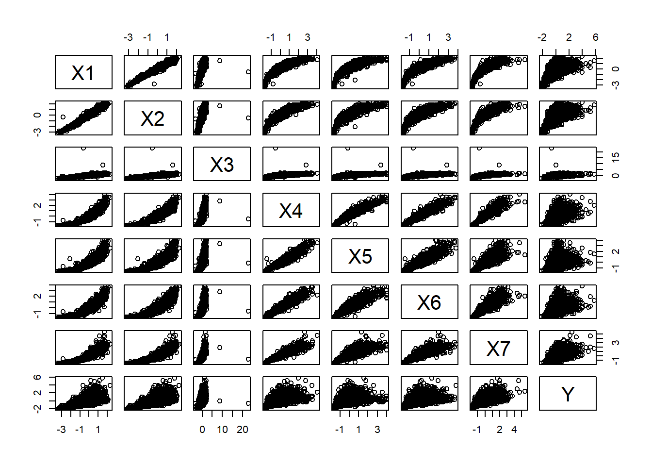
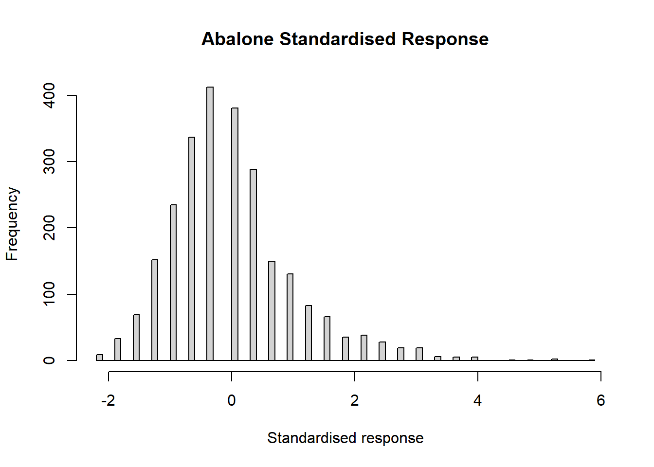
The age was found by counting the number of rings in the shell of the abalone, which leads to an integer response as can be seen from the digit preference of the histogram.
Linear Regression
A linear regression suggests that only the first feature, X1, is not predictive of Y
| term | estimate | std.error | p.value |
|---|---|---|---|
| (Intercept) | 0.000 | 0.014 | 1.0000 |
| X1 | -0.045 | 0.084 | 0.5887 |
| X2 | 0.414 | 0.084 | 0.0000 |
| X3 | 0.105 | 0.023 | 0.0000 |
| X4 | 1.459 | 0.144 | 0.0000 |
| X5 | -1.408 | 0.073 | 0.0000 |
| X6 | -0.371 | 0.058 | 0.0000 |
| X7 | 0.398 | 0.064 | 0.0000 |
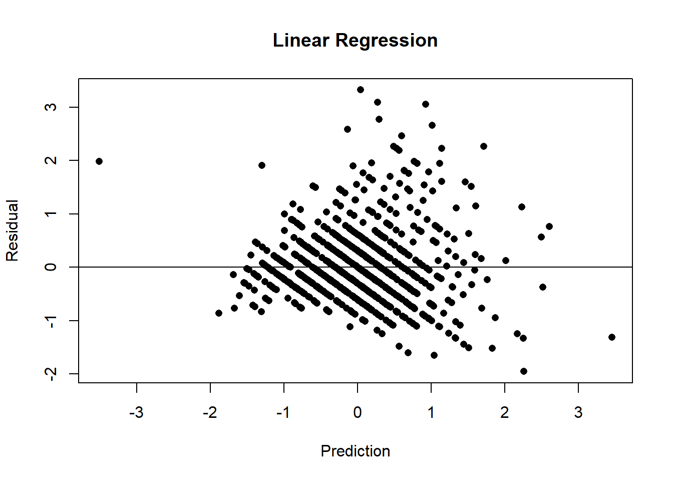
Using the prediction from this model, the residual mean square error (RMSE) in the validation data is 0.683. Because of the standardisation of the response this measure has characteristics that are very similar to R2 and it could reasonably be averaged across datasets. The baseline RMSE in the training data will be 1 and so the linear regression explains 100(1-RMSE2) or 53% of the variance. The residual plot below shows a striped pattern created by the integer nature of the unstandardised response and perhaps it also suggests that the variance is larger in older abalone.
XGBoost
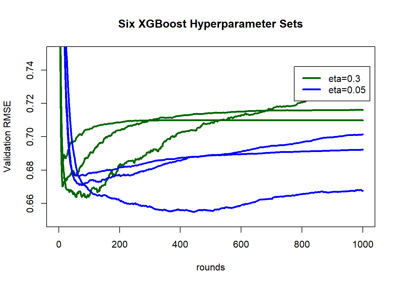
The XGBoost algorithm was run for 1000 rounds for each of six sets of parameters formed from crossing the learning rate (eta) equal to 0.05 or 0.2 and the maximum tree depth equal to 2, 6 or 9. A maximum tree depth of 6 is the default for the xgboost package.
| eta | max_depth | rounds | RMSE |
|---|---|---|---|
| 0.20 | 3 | 83 | 0.665 |
| 0.20 | 6 | 30 | 0.676 |
| 0.20 | 9 | 29 | 0.692 |
| 0.05 | 3 | 442 | 0.655 |
| 0.05 | 6 | 77 | 0.672 |
| 0.05 | 9 | 73 | 0.677 |
Bearing in mind that linear regression reduced the validation RMSE from 1 to 0.68 the performance of XGBoost is rather disappointing. The best set of hyperparameters only reduces the validation RMSE to 0.66 (0.655 in the table), this is equivalent to R2 of 57%, which is only 4% better than linear regression.
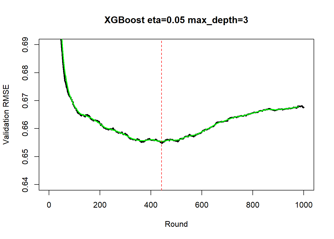
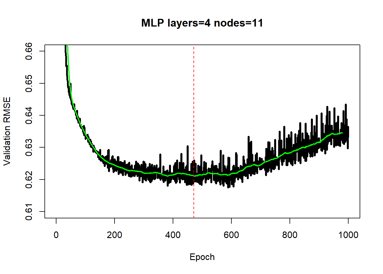
The next plot shows the history of the validation RMSE for the best combination of eta and max_depth (in black), overlaid with the smooth(in green). The optimum number of rounds is 442.
The history of the validation RMSE is shown below for each of the 6 sets of hyperparameters.
In this random split the model fits better to the test data (RMSE=0.639) than it did to the validation data(RMSE=0.655). As the validation RMSE is biased downwards due to it having selected for its low value, this is a little surprising. I expect that the selection bias is small and that the difference between 0.655 and 0.639 to be largely due to random splitting of the data, that is, it is an indication of the accuracy of the design. If the difference between validation and test samples (0.016) is a true indication of the possible sampling error, then we ought to be cautious about the selection of the optimal set of hyperparameters; eta=0.2 and max_depth=3 had a minimum validation RMSE of 0.665 which differs from the value for the selected best model by less than the validation/test difference.
MLP
The chosen hyperparameters for the MLP were the number of layers (2, 3 or 4) and the number of nodes per layer (fixed to be the same for every layer). The number of nodes was chosen dependent on the size of the training data so that there were either 5 observations per model parameter (weights + biases) or 20 observations per parameter. For the abalone data this meant either about 500 parameters or about 125 parameters.
| epochs | layers | nodes | parameters | RMSE |
|---|---|---|---|---|
| 416 | 2 | 18 | 505 | 0.625 |
| 355 | 3 | 13 | 482 | 0.623 |
| 471 | 4 | 11 | 496 | 0.621 |
| 601 | 2 | 7 | 120 | 0.623 |
| 980 | 3 | 6 | 139 | 0.626 |
| 274 | 4 | 5 | 136 | 0.631 |
For the MLP model the best set of hyperparameters is 4 layers of 11 nodes each run for 471 epochs. This model has 496 parameters, corresponding to approximately 5 observations per parameter (opp)) and the validation RMSE is 0.621 (R2=61%). The figure below shows the history of the validation RMSE. The stochastic nature of the adam algorithm creates the fluctuation in the RMSE and demonstrates the importance of the smooth, which overlaid in green.
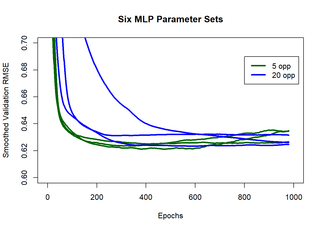
Below is the plot of the smoothed histories of all six MLP models. They all reach a similar performance level, but at different rates. Smaller models (opp=20, parameters=150) improve at a slower rate over the early epochs and their amount of overfitting by epoch 1000 is minimal.
Applying the selected MLP model of 4 layers of 11 nodes and 471 epochs to the test data gives a RMSE of 0.619 (R2=62%).
Based on the RMSE of the test data the “best” MLP out-performs the “best” XGBoost model by 0.020 (0.619 to 0.639) equivalent to an (R2 of 62% compared with 59%).
A Classification Task
The bank dataset comes from a Portuguese study in which people were contacted by telephone to encourage them to use a bank’s services. The response was whether or not the contact was successful.
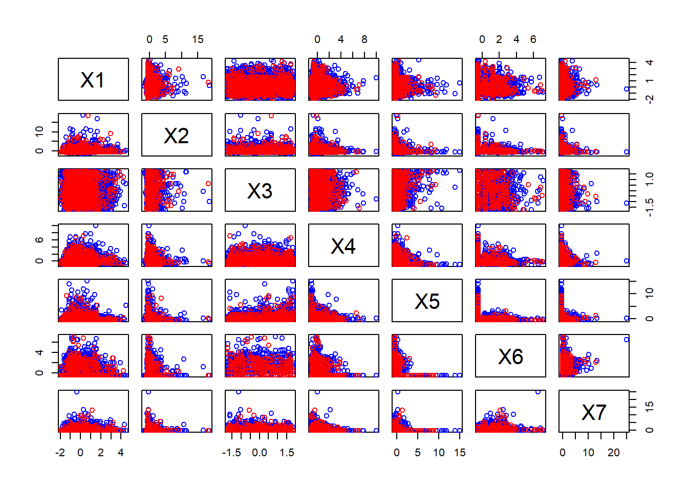
The plot shows the seven continuous standardised features with points plotted red if the contact was successful and blue if not. Several of the features are extremely skewed.
Logistic Regression
A basic logistic regression shows that only X1 fails to show linear association on the logit scale.
| term | estimate | std.error | p.value |
|---|---|---|---|
| (Intercept) | 0.223 | 0.033 | 0.0000 |
| X1 | 0.037 | 0.030 | 0.2156 |
| X2 | 0.220 | 0.034 | 0.0000 |
| X3 | -0.082 | 0.030 | 0.0067 |
| X4 | 1.735 | 0.054 | 0.0000 |
| X5 | -0.413 | 0.045 | 0.0000 |
| X6 | 0.257 | 0.036 | 0.0000 |
| X7 | 0.282 | 0.041 | 0.0000 |
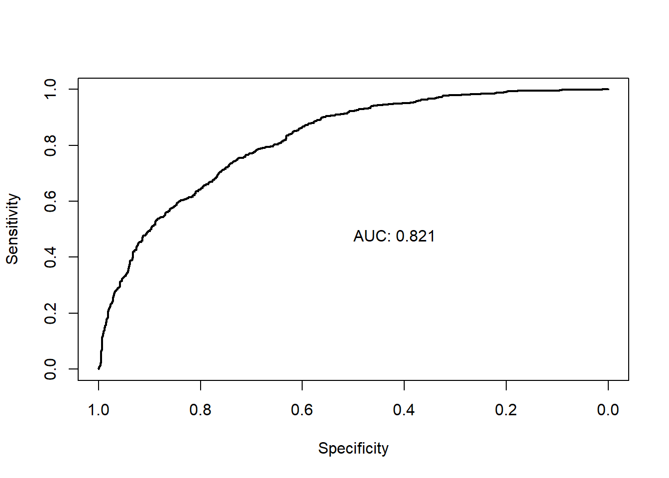
The ROC curve for logistic regression encloses an area of 0.82, which is the baseline for judging the performance of the more complex models.
XGBoost
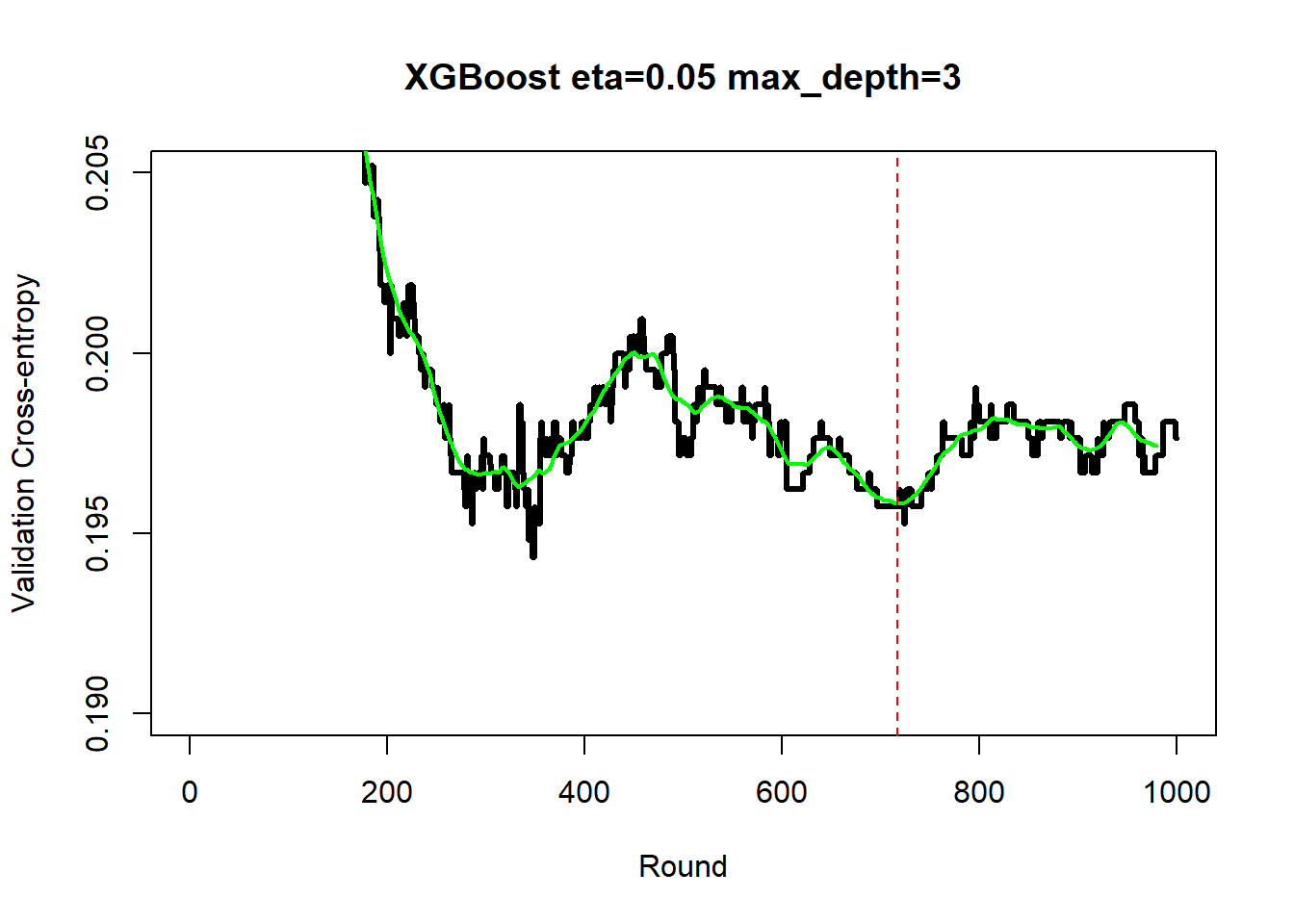
Six sets of predetermined hyperparameters were investigated and the minimum smoothed validation cross-entropy loss was 0.20, this was achieved when the learning rate was 0.05, the number of rounds was 717 and the maximum tree depth was 3. The AUC for this model in the test data was 0.88.
| eta | max_depth | Rounds | CE | AUC |
|---|---|---|---|---|
| 0.20 | 3 | 479 | 0.197 | NA |
| 0.20 | 6 | 39 | 0.198 | NA |
| 0.20 | 9 | 34 | 0.202 | NA |
| 0.05 | 3 | 717 | 0.196 | 0.875 |
| 0.05 | 6 | 600 | 0.197 | NA |
| 0.05 | 9 | 146 | 0.201 | NA |
| CE=Cross-Entropy | ||||
The plot below shows the history of the validation cross-entropy for the best of the six models. The history is much less smooth than for the regression example and as with all MLPs, it needs smoothing.
MLP
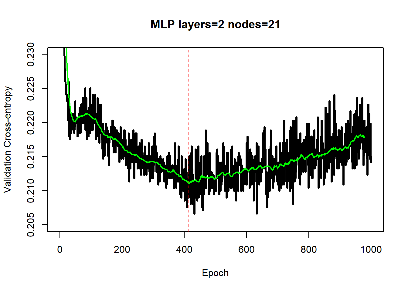
The best validation cross-entropy for the MLP models is 0.21, although all six complexities giving very similar performance. The test AUC for the best model was 0.86, compared with 0.82 for the logistic regression and 0.88 for XGBoost.
| opp | layers | nodes | NP | Rpochs | CE | AUC |
|---|---|---|---|---|---|---|
| 5 | 2 | 21 | 652 | 415 | 0.211 | 0.862 |
| 5 | 3 | 21 | 1114 | 30 | 0.221 | NA |
| 5 | 4 | 19 | 1312 | 110 | 0.220 | NA |
| 20 | 2 | 13 | 300 | 197 | 0.215 | NA |
| 20 | 3 | 10 | 311 | 236 | 0.215 | NA |
| 20 | 4 | 8 | 289 | 808 | 0.221 | NA |
| CE=Cross-Entropy | ||||||
The history of the validation cross-entropy shows the impact of the noise in the stochastic adam optimisation algorithm. Without smoothing the selection of the number of epochs would be unreliable as would be the estimate of the minimum cross-entropy.
Conclusions
Take care before jumping to any conclusions, these examples are meant to illustrate the workflow, they are not a substitute for the benchmarking itself. The examples were chosen alphabetically by the dataset name and not because they are in any sense typical. In my next post, I will show a summary of the results for all datasets and for all splits of the data.