Neural Networks: Torch in mlr3
Introduction
In this series, I am investigating how best to use artificial neural networks (ANNs) on tabular data and I am currently working towards a benchmarking experiment that will compare multi-layer perceptrons (MLPs) with XGBoost. In my last post, I introduced the torch R package, which provides an interface to the libtorch C++ library of functions for fitting ANNs. R’s torch closely mirrors PyTorch, Python’s popular interface to the same C++ library. In this post, I will show how to use torch within mlr3, an ecosystem of packages that facilitate complex machine learning experiments, such as benchmarking. This combination of packages relies heavily on a sub-project of mlr3 called mlr3torch that can be found on GitHub.
Both mlr3, torch and mlr3torch are all written using R6, a package that provides other package developers with the main features of Object Orientated Programming (OOP). R6 is used to define complex classes of R objects, so to use torch and mlr3 effectively it helps to understand how R6 objects are structured. A superficial knowledge of R6 will get you started, but my experience of using torch with mlr3 was that I needed a to know a little more.
R6 makes use of R environments. Before I started using mlr3torch I was vaguely aware of R’s environments from their use with functions and packages. Unfortunately, ‘vaguely aware’ proved insufficient, so I will start this post with a brief discussion of what more I needed to know about OOP, R6 and environments.
Preamble into R6
Object Orientated Programming
A decade or so ago OOP was all the rage, then fashions changed and there was a rise in the popularity of functional programming (FP). So it goes. Undoubtedly, there are problems that are well-suited to OOP and others that suit FP, so let’s start with a consideration of why OOP appeals to the developers of large, complex R packages.
OOP places the object at its centre and makes the OOP object into more than just a data structure. An OOP object does contain data stored in what are referred to as fields, but it also contains functions for accessing and manipulating those fields, in the jargon, these built-in functions are called methods. An OOP object’s fields and methods can either be public i.e. accessible to the user, or private, only available for internal use and hidden from the user.
When a user alters the contents of a field, directly if it is public, or indirectly via a public method if the field is private, those changes are performed in place, that is, the specified field changes and the previous value is lost.
OOP is a convenient way of organising complex data structures, which makes it a good choice for developing large packages; unfortunately, OOP is not part of the original design of R. The question that the developers of R6 had was, how do we get OOP behaviour within R? and their solution was to make use of R environments. Environments are R’s way of isolating collections of R objects from the rest of the workspace. They were originally intended for isolating the objects created within a function, but they can be adapted to provide a mechanism for mimicking OOP.
As an example of the more common use of the environment of a function, consider this code
f <- function(x) {
  y <- x + 1
  y * y
}
y <- 5
f(2)
On the last line, 2 is passed into the function f as argument x. Inside the function, one is added and the result, 3, is stored as y. The square of y is returned, so the result is 9. However, y already exists in the calling workspace with the value 5, so there is a clash of names. To sort out such clashes, R distinguishes between y in the global environment where it has the value 5 and y in the local environment of f where it has the value 3. In a sense, the local environment of f exists within the global environment, so we might refer to the global environment as the parent environment of f’s environment and since functions can call other functions in a long sequence, environments have a nested structure.
Suppose now that we were to change the code slightly, so that instead of adding 1 to x, we were to add y.
f <- function(x) {
  y <- x + y
  y * y
}
y <- 5
f(2)
When R comes to add y to x, there is no y within the function’s environment. A strict language would throw an error at this point and perhaps that would be for the best, but instead R searches in the parent environment to see if it can find y there. It does, so it calculates 2 + 5 and stores that as y local to f before returning 49. However, the y with the value 7 is within the function’s environment, it is not the same as the y in the parent environment, which still has the value 5.
Rant alert!
This is madness. the value of f(2) depends on the value of y somewhere in the hierarchy of environments that call f. If y changes in that far off environment, then the value returned by f(2) will change. No serious programmer would use such a language; you would be asking for deep, difficult to trace, bugs. In R’s defence, the language was designed for interactive statistical analysis, not large software projects.
Package developers could use a different strategy and treat R as an interface to OOP code written in a more appropriate language, such as C++, but that would come at a price, it would be difficult for the R user to dig down into the code. OOP via R6 is a compromise. Rant over, back to environments.
Even though there is rarely a need, it is possible to create an environment manually. The function that does this is env(), which is defined in the rlang package. Code for creating an environment called e might look something like
x <- 5
e <- rlang::env(
  a = c(1, 2, 3),
  b = "Fred",
  c = x
)
The contents of the environment are passed to env() as named arguments.
Printing an environment only gives its address in memory.
# print the environment with e, print(e) or str(e)
e
## <environment: 0x000001e022392858>Individual objects within an environment can be accessed using the same $ notation that is more commonly applied to lists.
# an object within the environment
e$a
## [1] 1 2 3The names of the items in the environment can be listed with names(e) or ls(e)
# names of items in the environment
names(e)
## [1] "a" "b" "c"The rlang function env_print() combines information from print() and names()
# names of items in the environment
rlang::env_print(e)
## <environment: 0x000001e022392858>
## Parent: <environment: global>
## Bindings:
## • a: <dbl>
## • b: <chr>
## • c: <dbl>Perhaps the best way to investigate the contents of an environment is the tree() function from the lobstr package
# an object with the environment
lobstr::tree(e)
## <environment: 0x000001e022392858>
## ├─a<dbl [3]>: 1, 2, 3
## ├─b: "Fred"
## └─c: 5Often software written with R6 includes environments nested within environments, so the tree can get very deep and complex, in that case, it can be helpful to set the max_depth argument oftree() to limit the print out.
Environments are very flexible, for example, as well as other environments, they can include functions and can even contain references to themselves. In the example, environment e2 includes a reference to environment e and to a function f.
# environment that references another environment
e2 <- rlang::env(
  e = e,
  f = function(x) x * x
)
lobstr::tree(e2)
## <environment: 0x000001e02204f078>
## ├─e: <environment: 0x000001e022392858>
## │ ├─a<dbl [3]>: 1, 2, 3
## │ ├─b: "Fred"
## │ └─c: 5
## └─f: function(x)The next block of code adds self to e2
# an environment that references itself
e2$self = e2
lobstr::tree(e2)
## <environment: 0x000001e02204f078>
## ├─self: <environment: 0x000001e02204f078> (Already seen)
## ├─e: <environment: 0x000001e022392858>
## │ ├─a<dbl [3]>: 1, 2, 3
## │ ├─b: "Fred"
## │ └─c: 5
## └─f: function(x)So e2$e is the same environment as e, and e2$self is the same environment as e2. Are these copies or merely references to original? Look at the addresses and you will see that the addresses are the same, so they are references. A simple experiment confirms that they are not independent copies. Changing e also changes e2$e.
# Changing e affects e2
e$b = "George"
lobstr::tree(e2)
## <environment: 0x000001e02204f078>
## ├─self: <environment: 0x000001e02204f078> (Already seen)
## ├─e: <environment: 0x000001e022392858>
## │ ├─a<dbl [3]>: 1, 2, 3
## │ ├─b: "George"
## │ └─c: 5
## └─f: function(x)Of course, it works both ways.
# Changing e2 affects e
e2$e$c = 18
lobstr::tree(e)
## <environment: 0x000001e022392858>
## ├─a<dbl [3]>: 1, 2, 3
## ├─b: "George"
## └─c: 18This means that we can add a reference to another environment without the memory cost of making a copy.
Let’s finish with a summary of a few key facts.
- any valid R object can be placed in an environment
- the objects in an environment are unordered and must be named
- environments can be nested
- nested environments save references not copies
- nested environments and their objects are referenced using the $ notation
Application to torch
In my last post, I turned a dataframe into a torch object using the code
library(torch)
# --------------------------------------------------------------
# Make a torch dataset from a dataframe
#
bike_dataset = dataset(

  name = "bike_dataset",

  initialize = function(df) {
    self$x <- torch_tensor(as.matrix(df[, -1]))
    self$y <- torch_tensor(as.matrix(df[, 1]))
  },

  .getitem = function(index) {
    list(x = self$x[index, ], y = self$y[index])
  },

  .length = function() {
    dim(self$x)[1]
  }
)
# --------------------------------------------------------------
# Create an instance of class bike_dataset called ds from data frame bdf
#
ds = bike_dataset(bdf)
bike_dataset is a class of object and ds is an instance, that is an actual R object with that class. Let’s dig into the object ds.
lobstr::tree(ds)## <environment: 0x000001e023d938f8>
## ├─y: S3<torch_tensor/R7>
## ├─x: S3<torch_tensor/R7>
## ├─.__enclos_env__: <environment: 0x000001e023d93c40>
## │ ├─.__active__: <list>
## │ ├─super: <environment: 0x000001e023dc2468>
## │ │ ├─clone: function(deep)
## │ │ ├─load_state_dict: function(x, ..., .refer_to_state_dict)
## │ │ ├─state_dict: function()
## │ │ ├─.getitem: function(index)
## │ │ └─.__enclos_env__: <environment: 0x000001e023dc2040>
## │ │ ├─.__active__: <list>
## │ │ └─self: <environment: 0x000001e023d938f8> (Already seen)
## │ └─self: <environment: 0x000001e023d938f8> (Already seen)
## ├─clone: function(deep)
## ├─.length: function()
## ├─.getitem: function(index)
## ├─initialize: function(df)
## ├─load_state_dict: function(x, ..., .refer_to_state_dict)
## └─state_dict: function()Given my preamble you will not be surprised to find that ds is an environment with a complicated structure, most of which was created by torch, but you will also find reference to the methods that my code added, initialize(), .getitem() and .length().
ds has inherited a function called state_dict(), we can look at it
ds$state_dict## function ()
## {
## fields <- names(self)
## tensors <- list()
## for (f in fields) {
## value <- .subset2(self, f)
## if (inherits(value, "torch_tensor")) {
## tensors[[f]] <- value
## }
## }
## tensors
## }
## <environment: 0x000001e023dc2040>and we can run it.
ds$state_dict()I have suppressed the output because this method returns the x and y fields and they are large. You should now also see the sense behind the references to self$x and self$y within initialize(). self is a reference to the environment itself, so it adds tensors called x and y to the main environment. The environment is the OOP object and x and y are its fields.
Do I need to know this?
We have been looking into details that most people would ignore. To use torch you only need to copy the pattern of the code for bike_dataset and adapt it to your particular problem. Perhaps, it is nice to know why you code self$, but after that you can leave the detail to the package developers.
So what do we need? Well, suppose that you were to run a linear regression with lm(). This function is written using the S3 class system and the results of the fit are returned in a list. An important skill for any R user is to be able to extract particular results from a returned list. With R6, the results are not returned in a list, rather they are added to an environment, so you will need to be able to extract the results from an environment. Often you will find that the developers have provided a method for extracting the data that you want, but other times they will not have, in which case you need to access the contents pf the environment for yourself.
Handling environments is to R6 what handling lists is to S3. In all other senses, you can leave the structure of R6 classes to the package developers.
mlr3
Enough preliminaries, it is time for mlr3. I have written about this package before in posts called Introduction to mlr3 and PipeOps in mlr3, so a brief recap will have to suffice as a preparation for incorporating torch.
mlr3 is an ecosystem of R packages and much like tidymodels, it automates the many stages in a machine learning analysis. Namely, data handling including preprocessing, model fitting, hyperparameter tuning and performance assessment. mlr3 is written using R6, a fact that can be ignored for routine use, but which becomes important for less standard work.
In a basic analysis, the user defines an R6 object to contain the data (this object is referred to as a task), another object defines the model (referred to as the learner), another the resampling scheme (the resampler) and another defines the performance assessment (the measures). Other classes cope with more complex needs such as a tuner for hyperparameter optimisation and a benchmark for organising a benchmarking experiment.
Quite often machine learning analyses are created by combining several steps, perhaps missing values are imputed, factors are encoded, the data are scaled and then the XGBoost algorithm is applied. In mlr3 such sequences are stored in pipelines using PipeOps and mlr3 ensures that the pipeline is used correctly, for instance by automatically ensuring that test data are scaled using statistics taken from the training data.
As an example of a simple analysis, I will take the Seoul Bike Sharing data that I analysed in my last post TensorFlow and PyTorch in R and I will fit a linear regression model to it using mlr3. I start with the data in a data frame called bdf that contains 14 features (predictors) and a single target (response) called count. The model is fitted to 80% of the data with the remaining 20% used for measuring the root mean square error. Finally predictions are made for the test data and the residuals are plotted against the predicted values.
As in my last post, the count has been transformed using log10(1+x).
# --------------------------------------------------------------
# Load the main packages of the mlr3 ecosystem
#
library(mlr3verse)

# --------------------------------------------------------------
# Turn bike data frame into a regression task
#
tsk_bike = as_task_regr(bdf, id = "bike", target = "count")

# --------------------------------------------------------------
# lm() is one of mlr3's standard learners
#
lrn_lm = lrn("regr.lm")
# --------------------------------------------------------------
# Use 80% for fitting and 20% for testing
#
set.seed(7802)
smp = rsmp("holdout", ratio = 0.8)
# --------------------------------------------------------------
# Run the analysis
#
rr = resample(tsk_bike, lrn_lm, smp)
## INFO [10:41:00.767] [mlr3] Applying learner 'regr.lm' on task 'bike' (iter 1/1)# --------------------------------------------------------------
# Select rmse as the performance measure & apply it to test data in rr
#
msr_rmse = msr("regr.rmse")
rr$score(msr_rmse)## task_id learner_id resampling_id iteration regr.rmse
## <char> <char> <char> <int> <num>
## 1: bike regr.lm holdout 1 0.3255388
## Hidden columns: task, learner, resampling, prediction_test# --------------------------------------------------------------
# Predictions for the test data
#
rrp = rr$prediction()
# --------------------------------------------------------------
# Residual Plot for test Data
#
y = rrp$truth
yhat = rrp$response
plot( yhat, y - yhat, pch=16,
xlab="Predicted", ylab="Residual", main="Regression Model")
abline(h=0)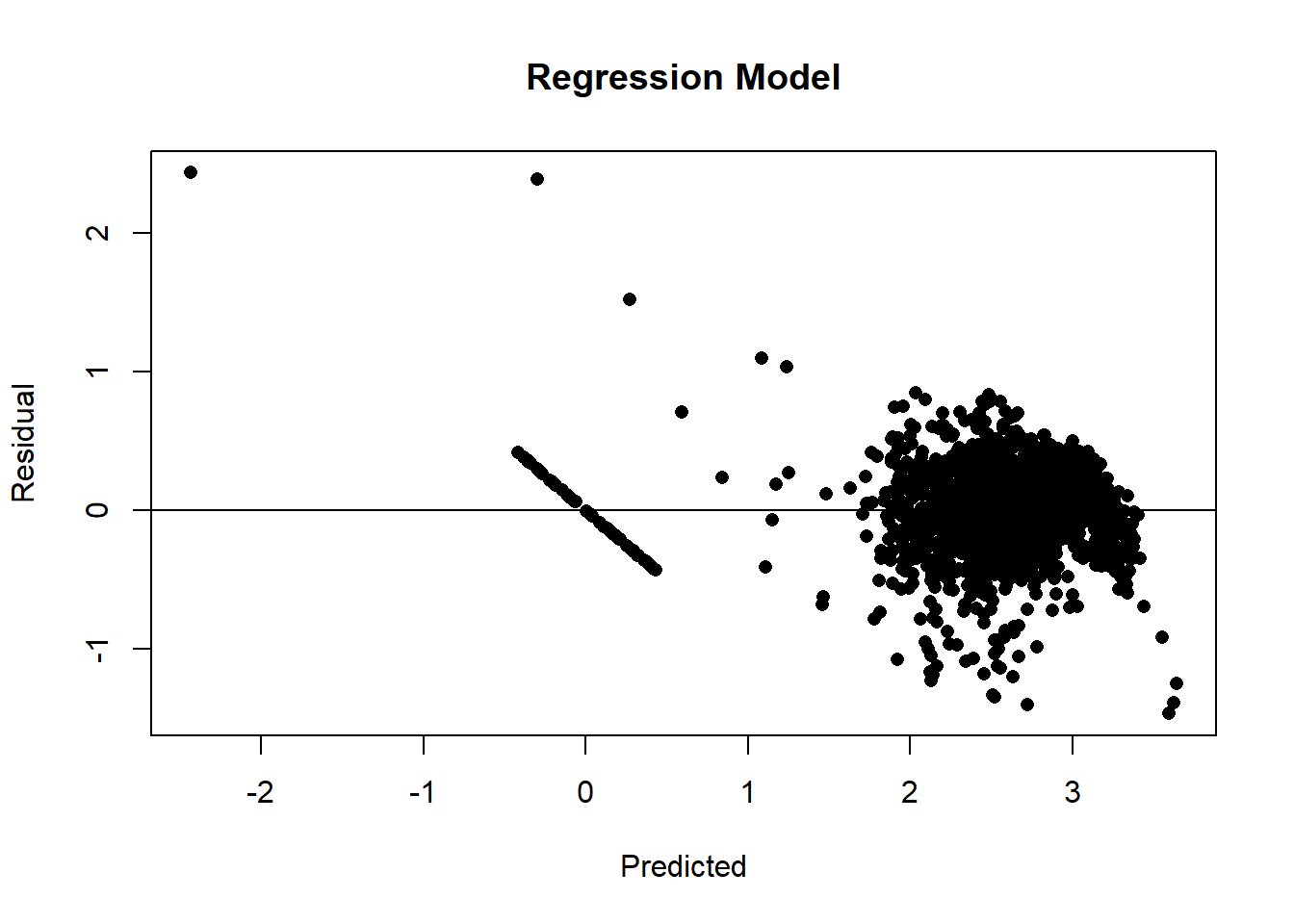
Disecting the results
The results of the analysis were stored in an object called rr. All of the results are in there, but how do we get at then? Well, rr is an environment created by R6 and we can discover its structure using a combination of two basic approaches,
- consulting the help files
- direct inspection of the environment
The help files
The mlr3 website includes a reference section that provides all of the information that you would get from R’s help system, for example by using ?resample. The webpage of information on resample can be found at https://mlr3.mlr-org.com/reference/resample.html. resample() is a function, so the help page starts with a list of possible arguments and follows with the return value, which we are told is an object of class ResampleResult. The description of the arguments of resample() uses several terms that are basic to the way that mlr3 works, so its is important to understand the jargon. These terms include,
- backend: the structure holding the data, typically a data.table
- encapsulate: run a function in a way that traps and stores all of the function’s warnings and messages
- hotstart: start fitting a model using starting parameter values obtained from a previous fit
- clone: make a copy
- umarshall: Serialisation is the process of turning an R object into a string of bytes so that it can be saved in a file, for example by using saveRDS(). Subsequently, the string of bytes can be read back from the file and the object reconstructed. Some R6 objects are so complex that the serialisation process fails, in which case the object needs to be marshalled prior to serialisation. The term marshall comes from an R package of that name that converts objects to a form that can be serialised. umarshall refers to the reverse process of unmarshalling.
- callbacks: extra calculations made at each iteration of the model fitting process; used to monitor progress.
The description of the class ResampleResult can be found at or from ?ResampleResult. Once again the key is to understand the terms used, which include,
- methods: The ResampleResult class has both S3 and R6 public methods. S3 methods are used in the conventional R fashion, for instance if rr is the name of an object of class ResampleResult, then the method as.data.table(rr) returns the results from rr as a data.table. In contrast, R6 methods are used with the $ notation, for instance rr$score(msr) applies a measure called msr to each of the resampled analyses.
- active bindings a binding is a name associated with a class’s field. When the data are fixed, the binding is static (its value does not change). However, in OOP, fields are changed in place, so a value associated with a field can change and the binding is said to be active. Imagine a class that stored a data.table, there might be a binding to the number of rows in the data. Were the data.table to be edited, this value would change, hence it would be an active binding.
Mapping the environment
The class structure used by mlr3 is described in detail in the help files, but since R6 classes are often referenced as elements within other R6 classes, tracing the information that you need can involve a lot of reading. Sometimes it is quicker to map the class structure in the way that I described in my preamble.
lobstr::tree(rr, max_depth=1)## <environment: 0x000001e02e08b428>
## ├─.__enclos_env__: <environment: 0x000001e02e08b0e0>...
## ├─errors: S3<data.table/data.frame>...
## ├─warnings: S3<data.table/data.frame>...
## ├─data_extra: S3<data.table/data.frame>...
## ├─learners: <list>
## │ └─<environment: 0x000001e03c0acb68>...
## ├─resampling: <environment: 0x000001e02ab72690>...
## ├─learner: <environment: 0x000001e03c48a078>...
## ├─task: <environment: 0x000001e02b315188>...
## ├─iters: 1
## ├─uhash: "1c535b37-a34a-4d61-b56a-c25c9441..."
## ├─task_type: "regr"
## ├─clone: function(deep)
## ├─set_threshold: function(threshold, ties_method)
## ├─unmarshal: function(...)
## ├─marshal: function(...)
## ├─discard: function(backends, models)
## ├─filter: function(iters)
## ├─aggregate: function(measures)
## ├─obs_loss: function(measures, predict_sets)
## ├─score: function(measures, ids, conditions, predictions)
## ├─predictions: function(predict_sets)
## ├─prediction: function(predict_sets)
## ├─help: function()
## ├─print: function(...)
## ├─format: function(...)
## └─initialize: function(data, view)Perhaps, you recognise some of the elements in the tree. Line 1 confirms that rr is an environment and gives its memory address. Further down the tree, you will see reference to environments for resampling, the learner and the task. These are active bindings and they are references to, not copies of, the environments for the R6 objects called tsk_bike, lrn_lm, smp that were created earlier in the code. There are also functions (R6 methods) such as score(), prediction(), that can be used to process the results.
Suppose that we wanted the coefficients of the linear model, where are they? Usually, the results of a model fit are placed in the class of the learner, Look at rr$learner$model and you will see that it is null. The model fit has not been saved.
rr$learner$model## NULLAn explanation can be found in the help files. resample() has an argument store_models that is FALSE by default. Had this argument been set to TRUE the model would have been saved as part of the resampling.
However, if you investigate rr$resampling and you will find the row numbers of the test and training sets. So, the model fit could be reproduced.
# -----------------------------------------
# Fit a linear model to the training data
#
lrn_lm$train(tsk_bike, row_ids = rr$sampling$instance$train)
# -----------------------------------------
# Inspect the fit
#
broom::tidy(lrn_lm$model)
## # A tibble: 15 × 5
## term estimate std.error statistic p.value
## <chr> <dbl> <dbl> <dbl> <dbl>
## 1 (Intercept) 2.56 0.00341 749. 0
## 2 day 0.00795 0.00345 2.31 2.10e- 2
## 3 dew 0.388 0.0368 10.6 7.11e- 26
## 4 func 0.496 0.00345 143. 0
## 5 holiday -0.0391 0.00345 -11.3 1.56e- 29
## 6 hour 0.123 0.00373 33.1 3.10e-226
## 7 humid -0.299 0.0155 -19.3 1.67e- 81
## 8 month 0.0831 0.00395 21.1 4.68e- 96
## 9 rain -0.104 0.00356 -29.4 9.26e-181
## 10 season -0.0607 0.00459 -13.2 1.91e- 39
## 11 snow -0.0121 0.00362 -3.35 8.00e- 4
## 12 solar -0.00189 0.00485 -0.389 6.97e- 1
## 13 temp -0.0963 0.0322 -2.99 2.78e- 3
## 14 visib 0.00600 0.00434 1.38 1.67e- 1
## 15 wind -0.00902 0.00389 -2.32 2.04e- 2This pattern is typical of mlr3. Provided that you follow a standard pattern of analysis, it is easy to use, but deviate slightly from the usual path and you will spend a long time searching through R6 data structures or countless help files to find the thing that you want. This is in part a weakness of R6 and in part a weakness in the design of mlr3, but at heart it is a limitation of R, or put more kindly, it is a result of using R for complex purposes that were not foreseen when R was designed.
mlr3torch
The pattern of an mlr3 analysis is simple and very flexible, we could easily replace the holdout resampling with cross-validation and get an analysis for each fold, or we could replace the linear model lm() with any of the other learners provided by mlr3. A list of mlr3’s learners is available by printing the mlr3 dictionary of learners.
library(mlr3learners)
library(mlr3extralearners)
lrns()
## <DictionaryLearner> with 176 stored values
## Keys: classif.abess, classif.AdaBoostM1, classif.bart,
## classif.bayes_net, classif.C50, classif.catboost, classif.cforest,
## classif.ctree, classif.cv_glmnet, classif.debug,
## classif.decision_stump, classif.decision_table, classif.earth,
## classif.featureless, classif.fnn, classif.gam, classif.gamboost,
## classif.gausspr, classif.gbm, classif.glmboost, classif.glmer,
## classif.glmnet, classif.IBk, classif.imbalanced_rfsrc, classif.J48,
## classif.JRip, classif.kknn, classif.kstar, classif.ksvm, classif.lda,
## classif.liblinear, classif.lightgbm, classif.LMT, classif.log_reg,
## classif.logistic, classif.lssvm, classif.mob,
## classif.multilayer_perceptron, classif.multinom, classif.naive_bayes,
## classif.naive_bayes_multinomial, classif.naive_bayes_weka,
## classif.nnet, classif.OneR, classif.PART, classif.priority_lasso,
## classif.qda, classif.random_forest_weka, classif.random_tree,
## classif.randomForest, classif.ranger, classif.reptree, classif.rfsrc,
## classif.rpart, classif.rpf, classif.sgd, classif.simple_logistic,
## classif.smo, classif.svm, classif.voted_perceptron, classif.xgboost,
## clust.agnes, clust.ap, clust.bico, clust.birch, clust.cmeans,
## clust.cobweb, clust.dbscan, clust.dbscan_fpc, clust.diana, clust.em,
## clust.fanny, clust.featureless, clust.ff, clust.hclust,
## clust.hdbscan, clust.kkmeans, clust.kmeans, clust.MBatchKMeans,
## clust.mclust, clust.meanshift, clust.optics, clust.pam,
## clust.SimpleKMeans, clust.xmeans, dens.kde_ks, dens.locfit,
## dens.logspline, dens.mixed, dens.nonpar, dens.pen, dens.plug,
## dens.spline, regr.abess, regr.bart, regr.catboost, regr.cforest,
## regr.ctree, regr.cubist, regr.cv_glmnet, regr.debug,
## regr.decision_stump, regr.decision_table, regr.earth,
## regr.featureless, regr.fnn, regr.gam, regr.gamboost,
## regr.gaussian_processes, regr.gausspr, regr.gbm, regr.glm,
## regr.glmboost, regr.glmnet, regr.IBk, regr.kknn, regr.km, regr.kstar,
## regr.ksvm, regr.liblinear, regr.lightgbm, regr.linear_regression,
## regr.lm, regr.lmer, regr.m5p, regr.M5Rules, regr.mars, regr.mob,
## regr.multilayer_perceptron, regr.nnet, regr.priority_lasso,
## regr.random_forest_weka, regr.random_tree, regr.randomForest,
## regr.ranger, regr.reptree, regr.rfsrc, regr.rpart, regr.rpf,
## regr.rsm, regr.rvm, regr.sgd, regr.simple_linear_regression,
## regr.smo_reg, regr.svm, regr.xgboost, surv.akritas, surv.aorsf,
## surv.bart, surv.blackboost, surv.cforest, surv.coxboost,
## surv.coxtime, surv.ctree, surv.cv_coxboost, surv.cv_glmnet,
## surv.deephit, surv.deepsurv, surv.dnnsurv, surv.flexible,
## surv.gamboost, surv.gbm, surv.glmboost, surv.glmnet, surv.loghaz,
## surv.mboost, surv.nelson, surv.parametric, surv.pchazard,
## surv.penalized, surv.priority_lasso, surv.ranger, surv.rfsrc,
## surv.svm, surv.xgboost.aft, surv.xgboost.coxYou might notice that torch is not one of the standard learners listed in the dictionary and given the flexibility and complexity of torch this is not surprising. However, there is a project called mlr3torch that is actively developing a learner for torch (https://github.com/mlr-org/mlr3torch).
The mlr3torch package is extensive and enables the creation within mlr3 of any artificial neural network that you can create in torch itself. Importantly though, there is are classes classif.mlp and regr.mlp that provide short cuts when the desired neural network is a multi-layer perceptron (MLP).
Let’s use the data in task tsk_bike to run a single holdout analysis of a MLP model, but with test and training data assigned manually.
First, we need to select 80% of the rows for training.
set.seed(5802)
train_ids = sample(1:nrow(bdf), 0.8*nrow(bdf), replace=FALSE)
test_ids  = setdiff( 1:nrow(bdf), train_ids)
Next. we set up the learner by adapting the class regr.mlp provided by mlr3torch.
library(mlr3torch)
lrn_mlp = lrn("regr.mlp",
  # define network parameters
  activation     = nn_relu,          # Activation Function
  neurons        = c(20, 10, 5),     # nodes in the hidden layers
  p              = 0,                # no dropout
  # training parameters
  batch_size     = 256,              # batch size
  epochs         = 150,              # number of epochs
  device         = "cpu",            # device
  # Proportion of data to use for validation
  validate       = 0.25,
  # Defining the optimizer, loss, and callbacks
  optimizer      = t_opt("adam"),
  loss           = t_loss("mse"),
  callbacks      = t_clbk("history"), # save results for each epoch
  # What to save each epoch
  measures_valid = msrs(c("regr.rmse")),
  measures_train = msrs(c("regr.rmse"))
)
Now we can fit the model to the training rows of bdf
# -----------------------------------------
# Fit the neural network
#
lrn_mlp$train( as_task_regr(bdf, row_ids = train_ids, target="count"))
The results are added to lrn_mlp so let’s search for them.
lobstr::tree(lrn_mlp, max_depth = 1)## <environment: 0x000001e02ba05000>## ├─.__enclos_env__: <environment: 0x000001e02ba05348>...
## ├─phash: "1b60375b2fa8293d"
## ├─hash: "90a1de1d5902ee2f"
## ├─param_set: <environment: 0x000001e02b7474d8>...
## ├─network: function(input)...
## ├─marshaled: FALSE
## ├─internal_tuned_values: <list>
## ├─internal_valid_scores: <list>
## │ └─regr.rmse: 0.22339379422543
## ├─callbacks: <list>
## │ └─<environment: 0x000001e029b1d118>...
## ├─optimizer: <environment: 0x000001e028b51510>...
## ├─loss: <environment: 0x000001e022045890>...
## ├─validate: 0.25
## ├─predict_types: "response"
## ├─selected_features_impute: "error"
## ├─hotstart_stack: <NULL>
## ├─encapsulation<chr [2]>: "none", "none"...
## ├─fallback: <NULL>
## ├─predict_type: "response"
## ├─errors<chr [0]>: ""
## ├─warnings<chr [0]>: ""
## ├─log: S3<data.table/data.frame>...
## ├─timings<dbl [2]>: 12.44, NA...
## ├─model: S3<learner_torch_model/list>...
## ├─data_formats: "data.table"
## ├─use_weights: "error"
## ├─man: "mlr3torch::mlr_learners.mlp"
## ├─timeout<dbl [2]>: Inf, Inf...
## ├─parallel_predict: FALSE
## ├─predict_sets: "test"
## ├─packages<chr [3]>: "mlr3", "mlr3torch", "torch"...
## ├─properties<chr [3]>: "internal_tuning", "marshal", "validation"...
## ├─feature_types<chr [3]>: "integer", "numeric", "lazy_tensor"...
## ├─task_type: "regr"
## ├─state: S3<learner_state/list>...
## ├─label: "My Little Powny"
## ├─id: "regr.mlp"
## ├─clone: function(deep)
## ├─initialize: function(task_type, optimizer, loss, callbacks)
## ├─dataset: function(task)
## ├─unmarshal: function(...)
## ├─marshal: function(...)
## ├─print: function(...)
## ├─format: function(...)
## ├─selected_features: function()
## ├─configure: function(..., .values)
## ├─encapsulate: function(method, fallback)
## ├─base_learner: function(recursive)
## ├─reset: function()
## ├─predict_newdata: function(newdata, task)
## ├─predict: function(task, row_ids)
## ├─train: function(task, row_ids)
## └─help: function()model seems a reasonable place to look, but I skip details of the search. The progress of the model fitting was saved in what mlr3 calls callbacks under the name history
lobstr::tree(lrn_mlp$model$callbacks$history, max_depth = 1)## S3<data.table/data.frame>
## ├─epoch<dbl [150]>: 1, 2, 3, 4, 5, 6, 7, 8, 9, 10, ......
## ├─train.regr.rmse<dbl [150]>: 2.30313836001785, 2.16549727075321, 1.84758628222725, 1.20238829281175, 0.660310555200954, 0.541535242650576, 0.484916621186495, 0.4492737198592, 0.422316339798797, 0.400610319535708, ......
## └─valid.regr.rmse<dbl [150]>: 2.25748706885577, 2.05399349475557, 1.55911758942807, 0.794025530529043, 0.590279657541638, 0.514033146118133, 0.470261285704779, 0.439050760522684, 0.413794711537539, 0.391694914323309, ......We have found the history and now we can plot it.
plot(lrn_mlp$model$callbacks$history$train.regr.rmse, col="red", type="l", lwd=2,
     ylim = c(0, 2), ylab = "RMSE", xlab="Epoch", main = "Architecture (14, 20, 10, 5, 1) ReLU Activation")
lines(lrn_mlp$model$callbacks$history$valid.regr.rmse, col="blue", type="l", lwd=2 )
legend(120, 1.8, legend=c("Train", "Valid"), col=c("red", "blue"), lwd=2)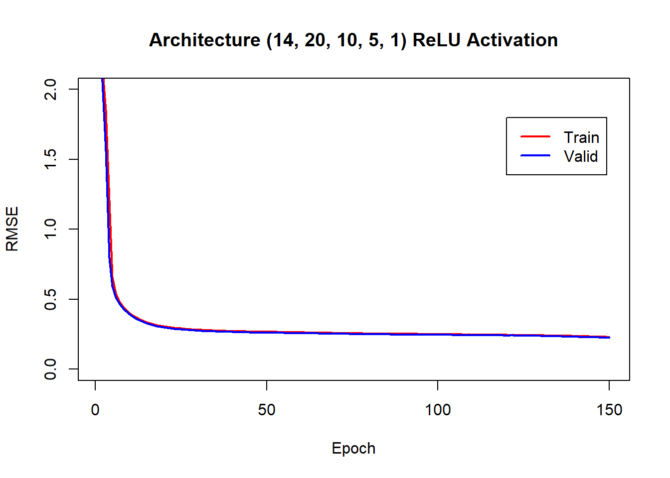
After making predictions for the test data, we can make a residual plot.
preds = lrn_mlp$predict(tsk_bike, row_ids = test_ids)

plot(preds$response, preds$truth - preds$response, pch=16, ylab="Residual",
     xlab="Predicted", main = "Test Data Predictions")
abline(h=0)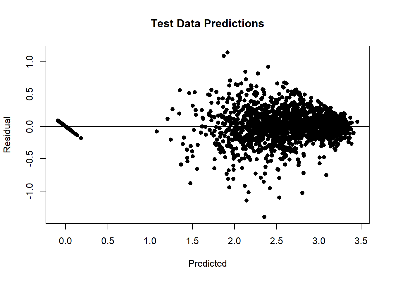
It is even more informative to plot the test data over time with the predictions superimposed.
plot(preds$row_ids, preds$truth, type="l", ylab="log10(count+1)", xlab="time",
     main="Model fit over time")
lines(preds$row_ids, preds$response, col="green")
legend(100, 0.65, legend=c("Actual", "Predicted"), col=c("black", "green"), lwd=2)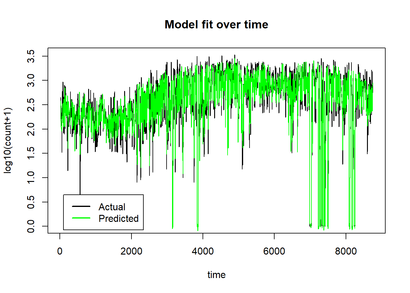
On the untransformed count scale the plot becomes,
plot(preds$row_ids, 10^preds$truth-1, type="l", ylab="Count", xlab="time",
     main="Model fit over time")
lines(preds$row_ids, 10^preds$response-1, col="green")
legend(100, 3200, legend=c("Actual", "Predicted"), col=c("black", "green"), lwd=2)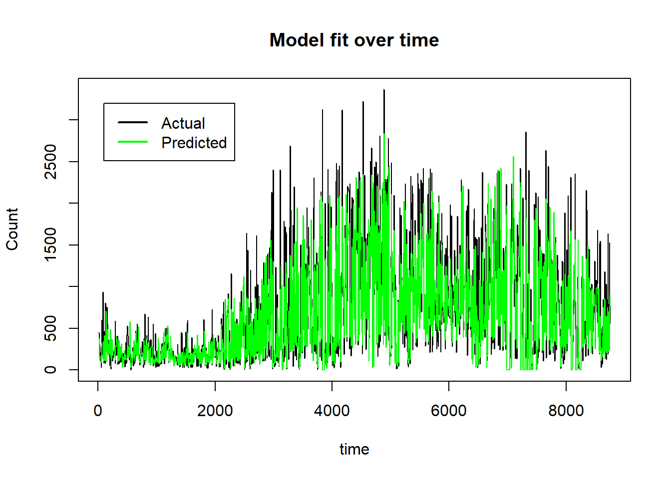
The neural network model has done a good job of picking up the non-linear trends over time and the interaction that puts the count to zero when the scheme is not functioning. Just how the model has done this is much less clear and there is still a good deal of work to be done to understand how the 14 features influence the model’s predictions. Within the paradigm of machine learning, prediction is king and understanding is secondary and by those standards, this is a good model.
Benchmarking
I am now quite close to being able to run the benchmarking experiment. mlr3 will organise the experiment and I have learners for the MLP and XGBoost models. What remains is to select some datasets for the experiment and to decide on the hyperparameters of the MLP and XGBoost models. In particular, do I tune the hyperparameters to fit each dataset? or, do I select default hyperparameters that perform reasonably over a range of datasets? Questions for my next post.
Final thoughts
mlr3 and torch are both excellent projects so I am reluctant to criticise them, but they leave me with the feeling that the developers have worked hard to compensate for basic limitations in R. Despite its age, I hope that it is not time for R to be retired, it still has many merits; it is very easy to learn, very flexible, excellent for interactive statistics, it has an amazing range of packages and there is an active and supportive community of users. To my mind, there is a problem when R is used for large projects, either the developers stick to R and find a solution that will be slow, error prone, artificial, labyrinthine, hard for the user to understand and difficult to maintain, or they create the project in a more appropriate language and use R as an interface to that code. Development in a second language seems to me to be the better option, but it means that the R users come up against a wall separating them from the underlying code. How do you give the R user full access to data manipulated in a second language? How do you give the R user the ability to adapt the code written in a second language? Perhaps, we we are approaching the time when statisticians will turn to a language that is better designed for modern use? Maybe, one that is similar to Julia.