Neural Networks: `TensorFlow` and `PyTorch` in R
Introduction
Apologies for the long gap between posts.
In this series, I am investigating how best to use artificial neural networks (ANNs) on tabular data and I am currently preparing a benchmarking experiment to compare multilayer perceptrons (MLPs) and XGBoost. In my last post, I reviewed some of the published literature on the performance of ANNs with tabular data and based on that review, I put forward two hypotheses that will underpin the benchmarking.
There always exists an MLP that models data as well as the best XGBoost model, the problem is finding it.
MLPs are less robust to messy data than is XGBoost, so preprocessing the data will make it easier to find the best MLP.
Admittedly these hypotheses still need refining to make them testable, but at least they give a sense of my direction of travel.
At the outset of my investigation of neural networks, I decided to write my own code for the fitting. Not only did this force me to develop a deeper understanding of the algorithms, but it also gave me the flexibility to experiment with whatever modifications seemed important at the time. When using someone else’s software, there is always the danger that you will merely reproduce the coder’s thought processes.
The downside of this independent approach is that my code is much less efficient than that used by most researchers and as a consequence I am limited to relatively small ANNs and small datasets. For the benchmarking, it would make sense to take advantage of one of the highly efficient R packages for fitting ANNs.
In this post, I will first compare TenssorFlow with Keras in R with the use of PyTorch in R and, spoiler alert, I will argue that PyTorch is the better option. I’ll then prepare the ground for using PyTorch in my benchmarking experiment, by presenting the code needed to fit a MLP.
Calculation and Interface
Fitting a Neural Network involves alternation between a forward and a backward algorithm. In the forward pass, the input values are passed through the layers of the network to produce predicted outputs and their corresponding loss. In the backward pass, the derivatives of the loss are found with respect to each of the model parameters starting with the derivatives of the loss itself and working back towards the parameters of the input layer. The forward pass reduces to a series of matrix multiplications and the backwards pass repeatedly applies the chain rule for differentiation to obtain the successive derivatives. The heart of any neural network software will be highly efficient code for computing with matrices plus code for applying the chain rule over a complex series of calculations.
While the forward calculation can be performed on matrices, it is sometimes more convenient to work with data in a three or higher dimensional array. In the jargon, an array with an arbitrary number of dimensions is known as a tensor, so the core code of an ANN library should be capable of tensor processing.
The key to improving the speed of the code will be parallel computation, both passes rely on the repeated application of the same pattern of calculations over multiple layers, either working forwards or backwards. There is much to be gained by parallel processing using the cores of the CPU, but even more to gain by using a GPU (Graphical Processing Unit). While a CPU will have, at best, a few tens of cores, a GPU has thousands of much simpler processing units.
On top of a tensor processing library, we will also need an interface in the form of software that is able to take the description of a neural network and turn it into a series of calls to the tensor processing library.
TensorFlow with Keras in R
In 2015, Google released a computational library called TensorFlow. As the name suggests, TensorFlow is a program for computing with tensors, i.e. multi-dimensional arrays. The algorithms that it uses are highly efficient and fast. TensorFlow will parallelise calculations and can use a GPU, if one is available. TensorFlow could be used for any array processing problem, but it has found its main applications in Machine Learning (ML), particularly deep learning and the fitting of ANNs. Indeed, it is now marketed as a tool for ML, even though it is more general.
TensorFlow works by organising the required array computations into a graph and then repeatedly computing over that graph. One big advantage of this structure is that it simplifies backpropagation of the derivatives of the loss; the chain rule is applied working backwards through the graph from loss to inputs.
Google provides several Application Programming Interfaces (APIs) that enable the user to specify their particular problem to TensorFlow. Keras is the high level API for specifying ANNs. Keras was first released at the same time as TensorFlow and has been under continual development ever since, of particular note is the release of Keras 3.0.0 in November 2023. Keras3 was a full rewrite of Keras which included the ability to to farm out the computation to packages other than TensorFlow. The current release (June 2025) is Keras 3.10
There is no R package for working directly with Keras or TensorFlow, but there are python packages that will do the job. R users have the reticulate package for communicating between R and python and thus they can indirectly use Keras and TensorFlow.
PyTorch in R
Torch is an open source library for computing with multi-dimensional arrays (tensors), it is fast and includes GPU acceleration. The original code was written in C with an interface written in the scripting language, Lua. Facebook, now Meta, adopted Torch and in 2016 released PyTorch, a Python interface for Torch, together with a version of Torch’s C code rewritten as a C++ library called libtorch. PyTorch/libtorch, quickly, became the method of choice for accessing the Torch library and from 2017 onwards, development of Torch stopped and effort was redirected into libtorch and its interface PyTorch.
Most computer languages are able to make use of libraries written in C or C++ and so interfaces to libtorch have been written for many languages including, Java, Rust, Julia, Haskell and R. Since the core of each of these is the same, it is possible to fit a model with torch in one language and then port the results for use in another language.
The R package torch is R’s equivalent of PyTorch, it provides an R interface to the libtorch C++ library and is capable of both direct tensor arithmetic and automatic differentiation. Sometimes people refer to torch for R as a version of PyTorch, but that is slightly misleading because torch for R does not use Python at all. This means that you can use torch in R without installing or knowing anything about Python.
Why I Prefer PyTorch
To use TensorFlow in R, you need to install TensorFlow, Keras, Python and R, plus the relevant Python and R packages. The CUDA software will also be needed for GPU acceleration. Installing Python and its packages will require you to first install the software management program Anaconda, or its smaller brother Miniconda. All of this would be a minor inconvenience were it not for the fact that the version numbers of every step in this software chain need to be compatible. Update one link in a working chain and you risk breaking your code.
The need to install Anaconda and Python is hard to justify unless you already use Python as well as R, in which case why not use Python for ypur deep learning. I have found that setting up TensorFlow from R is fiddly and that any working combination of the software is fragile.
In contrast, Torch just requires downloading the torch R package from CRAN and the running a single install_torch() function to set up the C++ library. You do still need to install a supported version of the CUDA software for GPU acceleration, but that is a minor problem.
I happen to like the mlr3 ecosystem for machine learning and use it in preference to tidymodels, which does much the same job. mlr3 has a project called mlr3keras that was developing a package for using Keras within its ecosystem. Development of this package stopped about three years ago, roughly the time when Keras3 was released. However, the mlr3torch, project which started much later is still under active development. Another reason for me to prefer PyTorch.
All that said, I do think that Keras has a better syntax with a clearer way of specifying the neural network and torch uses R6 which makes the syntax different from standard R. I have not run my own comparisons, but everything that I have read suggests that there is not much difference in speed between TensorFlow and PyTorch. The consensus opinion seems to be that TensorFlow is better for deployment and PyTorch is better for research; I do not have the experience to allow me to comment on that claim. Weighing up all of these considerations, PyTorch gets my vote, with my main consideration being that despite the name, PyTorch does not require Python.
An Introduction to PyTorch in R
The torch for R website (https://torch.mlverse.org/) is the main source of information on running PyTorch in R. The website has a very good companion book called Deep learning and Scientific Computing with R, which can be bought in paper form, or read on-line for free at https://skeydan.github.io/Deep-Learning-and-Scientific-Computing-with-R-torch/.
There are already a number of packages in the developing torch for R ecosystem
| R Package | What it does |
|---|---|
| torch | core interface to the libtorch C++ library |
| luz | An API that simplifies the specification of ANNs |
| torchvision | Functions for computer vision applications of ANNs |
| torchaudio | Functions for audio signal processing with ANNs |
| torchdatasets | Datasets for testing torch |
| ETM | word embeddings for language models |
| insight | functions for exploring deep learning models |
This is clearly a big topic, but in this post I’ll concentrate of the essentials for defining, fitting and predicting with a simple multilayer perceptron.
First, download the torch package from CRAN, run the package’s install_torch() function in the console and you are ready to go.
Working with R6 Classes
The torch R package is written using R6 classes. R6 is an R package that is used by many large R coding projects; for example, dplyr and mlr3 are both written using R6. Classes of Objects created with R6 have the properties needed for Object Orientated Programming (OOP). R6 objects have fields for storing data and methods, which are built-in R functions for manipulating the data in the fields.
Here is a hypothetical example of how an R6 object is created and used. Suppose that meta_analysis is an R6 class that I have written for processing meta-analyses. It has three fields n, mean and sd and four functions new(), fixed(), random() and addStudy(). Typical code might be
# data for a meta-analysis of two studies
df   <- data.frame((n=100,75), m=c(4.5, 4.3), s=c(6.3, 3.5))
# create a object of class meta_analysis with fields filled from df
BrCa <- meta_analysis$new(df)
# extract the contents of a field
BrCa$mean
# add an extra study to the meta-analysis
BrCa$addStudy(40, 4.2, 8.1)
# run a fixed effects meta-analysis
fma  <- BrCa$fixed()
In the jargon, BrCa is an instance of class meta_analysis and
changes to its fields happen in place, i.e. you do not need to make a copy of BrCa when you change the data, the fields themselves are changed.
As a user, you need to understand the $ notation. In the code above BrCa$mean is the name of a field, so the data in that field would have been printed, i.e. the vector 4.5, 4.3. However, BrCa$fixed(), with brackets at the end, refers to a method, i.e. an internal R function specific to that class. In the example, this function performs a fixed effects meta-analysis on the data in the fields and returns the result as a list of calculated values. All R6 objects are created by a method, conventionally called, new().
Preparing the Data for Torch
We are going to use the torch software for processing the tensors that contain the data and parameters of our ANN. Torch’s code is optimised for speed, part of which comes from the way that the tensors are stored in memory. The arrays are typically large and the libtorch code needs to be able to retrieve batches of data from the arrays so that they can be processed in parallel.
A typical pattern is to start with data in an R data frame and to convert it into torch tensors, but there are two limitations on the data that can be placed in a tensor that do not apply to data frames.
- Torch tensors can only contain numeric data (no character strings, booleans or factors)
- Torch tensors cannot contain missing values
When necessary, you will need to write R code that manipulates your data into numeric form without missing values by encoding strings, booleans and factors and imputing missing data. This requires standard R code, so I’ll park these problems until we come to look at an example.
The torch package provides an R6 class called dataset that stores your data as a tensor and makes it available to the tensor processing functions. Although, torch does much of the work, there are things about your data that the package cannot anticipate, so you will need to supply extra information to complete the class definition. In particular, you need to supply three methods with the names initialize(), .getitem() and .length(). The first is used by new() when an instance is created, the second returns a single row of data given its row number and the third returns the number of observations in the dataset. The code that you need to write will look something like this,
ds_class <- dataset(
  initialize = function(...) {
    ...
  },
  .getitem = function(index) {
    ...
  },
  .length = function() {
    ...
  }
)
This code creates a completed R6 class called ds_class that inherits the fields and methods of dataset, but adds the methods that you provide.
To make the example more concrete, suppose that the data are in an R data frame and that the first column is the response and the other columns are numeric predictors.
ds_class = dataset(
  name = "my_dataset_class",
  initialize = function(df) {
    self$x <- torch_tensor(as.matrix(df[, -1]))
    self$y <- torch_tensor(df[, 1])
  },
  .getitem = function(index) {
    list(x = self$x[index, ], y = self$y[index])
  },
  .length = function() {
    dim(self$x)[1]
  }
)
To the standard class dataset provided by torch, I have added a field called name and the three required methods. Initialize() takes a data frame as its input and converts the numeric R values into arrays of torch tensors with the field names self$x and self$y. The same data as in the data frame, but stored as torch tensors. df is the name of an argument to the function, it is not an actual R data frame.
.getitem() takes an index (row number) and returns a list containing the predictors and response for that row. .length() returns the number of rows.
ds_class is a class derived from the more general class dataset , it is not an instance of that class. When we create the instance (actual object) we will put some data into it. To create an instance called, ds, I call ds_class with the name of an actual R data frame, represented here by real_df.
ds <- ds_class(real_df)Dataloader
Once you have defined the dataset, you must create a dataloader, which torch will use to access batches of data. In the code below, the rows of data in ds will be shuffled before batches of size 10 are taken. This means that each iteration will split the dataset in a different way, so avoiding any patterns associated with a meaningful ordering of the data.
dl <- dataloader(ds, batch_size = 10, shuffle = TRUE)The dataloader will extract batches of the required size, using the .getitem() method that you defined. Class dataloader has many predefined methods such as dataloader_next() which extracts the next batch of data and keeps track of your current position in the dataset by updating a field that contains a pointer into the data. All of this is done for you using highly efficient code.
Defining the Model
So far we have only used the torch package, for the next step we will need the companion package luz that enables you to turn a neural network architecture into a form that torch can process.
luz is also written using R6, so you will not be surprised to find that you must create an instance of a model class, which luz gives the name nn_module. luz does most of the work for you, but there are some things that the package cannot anticipate, such as the specific model architecture that you want to use, so you will have to add to the definition, just as you did with the dataset. This time you need to supply two methods initialize() that defines the components of the network and forward() that describes how the model takes input values and produces an output. This is far easier than it sounds because luz provides a wide range of functions for defining layers and activation functions, all that the user needs to do is combine them like the pieces of a jigsaw.
Here is a simple example that defines a neural network with an input layer, a single hidden layer with 10 nodes and an output layer. The hidden layer incorporates a sigmoid activation function. All of the functions beginning nn_ or nnf_ are provided by luz and self refers to one of the field within the class.
net <- nn_module(
  initialize = function(nInput, nOutput) {
    self$fc1 = nn_linear(nInput, 10),
    self$fc2 = nn_linear(10, nOutput)
    )
  },
  forward = function(x) {
    x |>
      self$fc1() |>
      nnf_sigmoid() |>
      self$fc2()
  }
)
initialize() defines two sets of parameters, one for connecting the input layer to the hidden layer and one for connecting the hidden layer to the output layer. Layers defined by nn_linear() are fully connected (dense), hence the conventional use of fc in their name; you could call them anything you like, but they have to be defined as being within self. forward() puts the layers together in the required order and adds any activation functions. The use of the pipe |> makes the structure clearer.
In the example, net is an R6 class with two hyperparameters which need to be specified when we create an instance, these hyperparameters are nInput, the number of nodes in the input layer and nOutput, the number of nodes in the output layer. The number of nodes in the single hidden layer is hard-coded into the design.
Training
Training is easier than the definition of the model, because the specification is less problem specific and luz does most of the work for you.
fitted <- net |>
  setup(loss = nn_mse_loss(), optimizer = optim_sgd) |>
  set_hparams(nInput = 5, nOutput = 1) |>
  set_opt_hparams(lr = 0.05) |>
  fit(dl, epochs = 50)
net is the R6 class derived from nn_module, this is piped into the luz function setup() that adds the loss function and optimizer. There are many options provided by luz, I’ve chosen the mean square error loss and the Stochastic Gradient Descent (SGD) optimizer. Both the architecture of the network and that of the optimizer rely on hyperparameters, so these are specified in set_hparams() and set_opt_hparams() respectively. lr is the learning rate for the SGD algorithm.
The network is initialised with random weights and biases and refined over 50 epochs, or iterations, of the SGD algorithm.
Enough, this is the basic pattern, we are now ready for an example.
Seoul Bike Sharing Demand
For this example, I took the bike sharing data from the UCI Machine Learning Repository https://archive.ics.uci.edu/dataset/560/seoul+bike+sharing+demand. These data can also be found as a kaggle dataset. Our task is to predict the number of bikes hired during each hour of each day during 2020, using data on the weather conditions at the time.
Reading these data is not totally straightforward because the header in the csv file includes non-ASCII characters and unquoted spaces.
library(torch)
library(luz)

home = "C:/Projects/Neuralnets/Torch"

# --------------------------------------------------------------
# Read data file as character strings
#
txt = readLines(file.path(home, "data/rawData/SeoulBikeData.csv"))
# --------------------------------------------------------------
# Remove non-ascii characters
#
txt = iconv(txt, from = "UTF-8", to = "ASCII", sub = "")
# --------------------------------------------------------------
# Strings are not quoted. Replace space with underscore
#
txt = gsub(" ", "_", txt)
# --------------------------------------------------------------
# Read the strings as a csv file & save in a data frame
#
bdf = read.csv(textConnection(txt), header=TRUE)
The column names are long and irregular, so I rename them with shorter versions. count is the column that I want to predict.
# --------------------------------------------------------------
# Short column names
#
names(bdf) = c("date", "count", "hour", "temp", "humid", "wind", "visib",
              "dew", "solar", "rain", "snow", "season", "holiday", "func")
From the date column, which is currently a string variable, I decided to extract the month, and the day of the week.
# --------------------------------------------------------------
# Convert date & replace by day of week and month number
#
bdf$date   = as.Date(bdf$date, "%d/%m/%y")
bdf$day    = weekdays(bdf$date)
bdf$month  = as.numeric(format(bdf$date, "%m"))
After plotting the total counts for each day, the date itself is dropped from the data frame.
totals     = aggregate(bdf$count, by=list(bdf$date), sum)
plot(totals$`Group.1`, totals$x, type="l", ylab="Daily Total", xlab="Day",
     main="Bikes hired each day")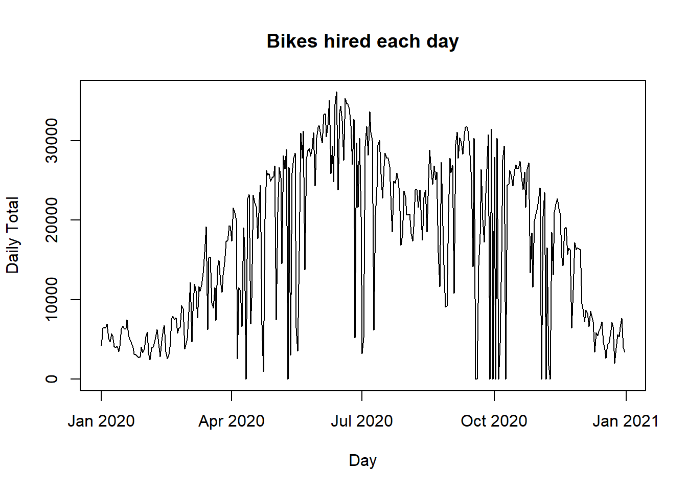
bdf$date = NULLThe plot shows that bike sharing is low in the winter, drops to zero on days when the scheme is not functioning, drops slightly in August presumably due to annual holidays. It also shows a weekly pattern with dips at the weekend.
Next, I convert all of the factors to integers, preserving any meaningful ordering. I decided that changes in bike usage are likely to be proportional rather than additive, so I log transformed the count (proof, if proof were needed, that I’m a statistician at heart and not a data scientist).
# --------------------------------------------------------------
# Replace strings by integers
#
bdf$season = as.numeric(
  factor(bdf$season, levels=c("Spring", "Summer", "Autumn", "Winter")))
bdf$holiday = as.numeric(
  factor(bdf$holiday, levels=c("No_Holiday", "Holiday")))
bdf$func = as.numeric(
  factor(bdf$func, levels=c("No", "Yes")))
bdf$day = as.numeric(
  factor(bdf$day, levels=c("Monday", "Tuesday", "Wednesday", "Thursday",
                          "Friday", "Saturday", "Sunday")))
# --------------------------------------------------------------
# Log transform the response
#
bdf$count = log10(1 + as.numeric(bdf$count))
Now that all data are numeric, I can scale the entire dataset. This makes no difference to the neural network, other than ensuring that the weights and biases are all of the same order of magnitude, which makes model fitting easier.
# --------------------------------------------------------------
# Scale features
#
bdf[, 2:15]   = scale(bdf[, 2:15])
Now we start the neural network analysis by defining the bike_dataset class and an instance of the class called bds.
# --------------------------------------------------------------
# Make a torch dataset from a dataframe
#
bike_dataset = dataset(
  name = "bike_dataset",
  initialize = function(df) {
    self$x <- torch_tensor(as.matrix(df[, -1]))
    self$y <- torch_tensor(as.matrix(df[,  1]))
  },
  .getitem = function(index) {
    list(x = self$x[index, ], y = self$y[index])
  },
  .length = function() {
    dim(self$x)[1]
  }
)

# --------------------------------------------------------------
# Create an instance of class from data frame bdf
#
bds = bike_dataset(bdf)
I’ll randomly divide the data into a training set (60%), a validation set (20%) and a test set (20%). I have been slightly lazy, because the scaling should have been performed using the mean and standard deviation of the training data. The effect of not doing this will be to improve performance of the validation and test samples, but only very slightly and doing it properly would make the code more messy. It is just the sort of thing that mlr3 is intended for.
# --------------------------------------------------------------
# Split between training, validation and test
#
set.seed(4682)
train_ids = sample(1:length(bds), size = 0.6 * length(bds))
valid_ids = sample(setdiff(1:length(bds), train_ids), size = 0.2 * length(bds))
test_ids  = setdiff(1:length(bds), union(train_ids, valid_ids))

train_ds  = dataset_subset(bds, indices = train_ids)
valid_ds  = dataset_subset(bds, indices = valid_ids)
test_ds   = dataset_subset(bds, indices = test_ids)
Next we need dataloaders for the three datasets. Shuffling the training data protects against any patterns in the batches that are drawn. This is important because most training algorithms calculate gradients on a sample of the data and it would be dangerous to rely on consecutive rows. Shuffling is not needed for the validation and test data, because we only make predictions and those predictions are for the entire sample, even if it is calculated in batches.
# --------------------------------------------------------------
# Create dataloaders
#
train_dl = dataloader(train_ds, batch_size = 200, shuffle = TRUE)
valid_dl = dataloader(valid_ds, batch_size = 200, shuffle = FALSE)
test_dl  = dataloader(test_ds,  batch_size = 200, shuffle = FALSE)
The neural network that I will use is defined by class NN5. As well as the input and output layers there are three hidden layers with 20, 10 and 5 nodes respectively. Five layers means four sets of parameters connecting the layers.
# --------------------------------------------------------------
# NN5 a Class of NN model with 5 layers
#
NN5 = nn_module(
name = "five_layer_model",
initialize = function(nInputs, nOutputs) {
self$fc1 = nn_linear(nInputs, 20)
self$fc2 = nn_linear(20, 10)
self$fc3 = nn_linear(10, 5)
self$fc4 = nn_linear(5, nOutputs)
},
forward = function(x) {
x |>
self$fc1() |>
nnf_sigmoid() |>
self$fc2() |>
nnf_sigmoid() |>
self$fc3() |>
nnf_sigmoid() |>
self$fc4()
}
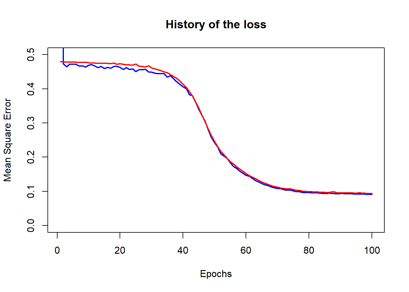
)Fitting will be by stochastic gradient descent over 100 epochs with a learning rate of 0.05. The mse loss is monitored in both the training and the validation data.
nEpoch = 100
torch_manual_seed(4751)

NN5_fit = NN5                             |>
  setup(loss      = nn_mse_loss(),
        optimizer = optim_sgd )           |>
  set_hparams(nInputs = 14, nOutputs = 1) |>
  set_opt_hparams(lr = 0.05)              |>
  fit(train_dl, epochs = nEpoch, valid_data = valid_dl)
Extracting and plotting the history of the MSE loss shows that it drops to just below 0.1.
We can compute the predictions in the validation data and plot residuals against fitted values. The predictions are returned as a tensor and then converted to an R numeric variable.
preds <- as.numeric(predict(NN5_fit, valid_dl))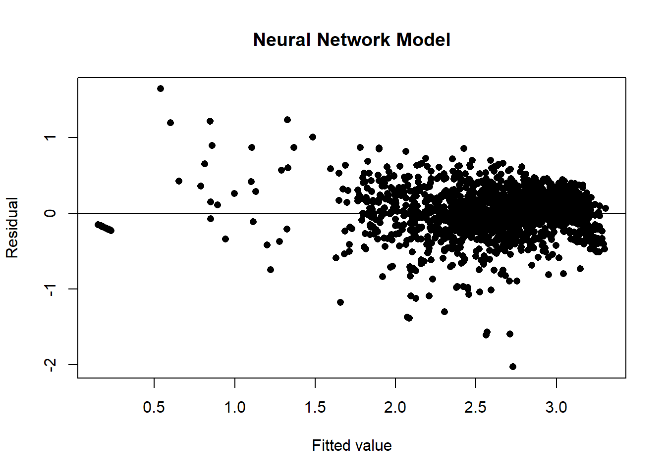
Where we to use the validation sample to select the hyperparameters, network architecture or the number of epochs, then we could estimate the performance of the chosen model using the test sample.
Linear Regression
For comparison, here are the results of a standard linear regression. The residual plot shows evidence of patterns that the model has not captured, however the ANOVA has a residual mean square error that is just over 0.1; only slightly worse than the neural network.
m = lm(count ~ ., data = bdf)
yhat = predict(m)
plot(yhat, bdf$count - yhat, pch=16, ylab="Residual", xlab="Fitted value",
     main = "Linear Regression")
abline(h=0)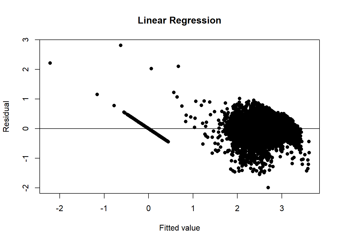
## Analysis of Variance Table
##
## Response: count
##             Df  Sum Sq Mean Sq    F value    Pr(>F)
## hour         1  297.92  297.92  2919.6690 < 2.2e-16 ***
## temp         1  465.77  465.77  4564.6523 < 2.2e-16 ***
## humid        1  205.11  205.11  2010.0909 < 2.2e-16 ***
## wind         1    6.00    6.00    58.8034 1.929e-14 ***
## visib        1    0.04    0.04     0.3797   0.53778
## dew          1   14.67   14.67   143.7990 < 2.2e-16 ***
## solar        1    0.28    0.28     2.6976   0.10054
## rain         1   85.44   85.44   837.3290 < 2.2e-16 ***
## snow         1    0.03    0.03     0.2739   0.60072
## season       1   28.52   28.52   279.4555 < 2.2e-16 ***
## holiday      1   19.96   19.96   195.6249 < 2.2e-16 ***
## func         1 2059.13 2059.13 20179.7205 < 2.2e-16 ***
## day          1    0.40    0.40     3.8784   0.04894 *
## month        1   45.24   45.24   443.3831 < 2.2e-16 ***
## Residuals 8745  892.33    0.10
## ---
## Signif. codes:  0 '***' 0.001 '**' 0.01 '*' 0.05 '.' 0.1 ' ' 1
Given that the neural network is not much of an improvement on linear regression, we might be tempted to increase the size of the network, try other activation functions or different optimisation algorithms. I will not show the details, but it is easy to get the validation MSE below 0.07.
Appendix: Earlier posts
My earlier posts in this series have covered, R code for fitting a neural network by gradient descent, Rcpp to convert the R code to C for increased speed, picturing gradient descent search paths, using neural networks to simulate datasets for use in my experiments, first steps towards a workflow, the pros and cons of cross-validation, extending the workflow to include classification problems, class assignment after classification, regularisation and overfitting, stochastic gradient descent
There are numerous other posts relating to statistics and its relationship with machine learning.