Neural Networks: Stochastic Gradient Descent
Introduction
In this series of posts, I am developing a workflow for using neural networks in data analysis. So far, I have
- written R code for fitting a neural network by gradient descent
- used Rcpp to convert the R code to C for increased speed
- pictured gradient descent search paths
- used neural networks to simulate datasets for use in my experiments
- made some tentative first steps towards a workflow
- considered the pros and cons of cross-validation
- extended the workflow to include classification problems
- defined and experimented with regularisation
This post introduces the stochastic gradient descent algorithm a method that makes neural network fitting practical for large datasets. The code that I used to implement SGD is available on my GitHub pages.
What is Stochastic Gradient Descent
Even at the best of times, gradient descent (GD) is a slow algorithm, but when a neural network (NN) is fitted to a large set of training data, GD can almost grind to a halt. Each iteration of the algorithm cycles through every observation in the training data and runs a forward pass to calculate the value of each node and a backward pass to find the gradients. The amount of computation is proportional to the size of the training set and to the number of nodes.
Since computation for GD involves independent calculations for each observation in the training data, the algorithm is an ideal candidate for parallel processing, but in this post, I will only consider how the speed can be improved when the algorithm is run as a single process.
The gradients used in GD are obtained by summing the results for each training observation. This suggests a simple way of speeding up the calculation; make the calculations for a random sample of the training data and scale up the sum of the gradients proportionately. Each iteration will take a fresh random sample from the training data, so if one time the gradient estimates are misleading, the algorithm should quickly recover. The gradients derived in this way will be less accurate than those of full GD, but the computation will be much quicker. The hope is that faster computation will allow more iterations and compensate for the loss in accuracy.
In pure stochastic gradient descent (SGD), the gradients are calculated from a single random observation drawn from the training data. Extreme as it might sound, pure SGD will converge, although the gradients can vary wildly and a small step length may be needed to stop the algorithm from diverging.
Basing the gradient estimates on a larger sample from the training data is called mini-batch SGD. Each iteration will involve more computation than pure SGD, but the algorithm should be much more stable. The fact that pure SGD works at all, tells us that the sample size for mini-batch SGD can be very small.
Full gradient descent can be likened to a skier taking the quickest route down a mountain, while stochastic gradient descent slaloms from side to side.
Epochs and iterations
For the gradient descent (GD) algorithm, my code calculates both the gradients and the loss at every iteration, this makes sense as the computation of the gradients provides all of the information needed to evaluate the loss.
With stochastic gradient descent (SGD) the situation is different because the gradients are only calculated for a sample of the training data and evaluating the corresponding loss would mean a forward pass of all of the omitted training data, which would remove much of the gain. Instead, my code only evaluates the loss on the full data after M sample-based parameter updates, where M is a value specified by the user. The gradient-based updates and the loss evaluation are working on different time scales, so which do you call an iteration?
Machine learning terminology seems to vary from user to user, but my choice is to say that the loss is evaluated once per Epoch and the gradients are estimated once per iteration. So if the gradients are estimated M times per epoch, the total number of iterations = number Epochs * M. I’ll refer to M as the number of batch iterations, meaning the number of gradient-based updates within each epoch.
There are two ways to select batches of size B, systematically or randomly. You could work through the training data taking the first B rows, then the next B rows and so on, but this would be dangerous because the order of the rows sometimes has meaning, perhaps it reflects the order in which the data were collected. Any such ordering could create unhelpful patterns in the gradients and so it is safer to choose the batches randomly.
A simple way to implement random mini-batch selection is to chose a batch size, B, out of the N possible training observations and then to run through each training observation in turn and include it in the gradient calculation based on a probability. If, so far, b observations have been used in the gradient calculation and n observations have been considered, then B-b more gradients will be needed to complete the batch and N-n observations will be left for possible inclusion. The next observation should be included with probability (B-b) / (N-n).
There is much more to say about SGD, but a simple illustration will help highlight the key properties.
Hump: A simple example
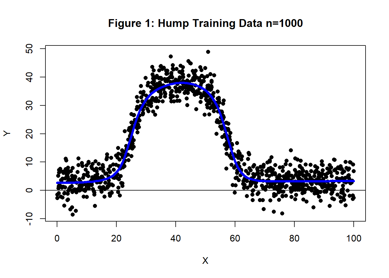
I generated training data with n=1,000 from a curve that I’ll call the Hump. The simulation was such that the RMSE of a model that perfectly identifies the trend would be four. Figure 1 shows a plot of the the training data and the curve used to generate it. This hump dataset will be analysed using a (1, 4, 1) neural network first by GD and then by SGD.
Gradient Descent
When comparing SGD to gradient descent (GD), it is important to ensure that both algorithms use well-chosen step lengths, because step length has a big impact on the speed of convergence. Figure 2 shows the histories of three GD analyses of the hump data using different fixed step lengths.
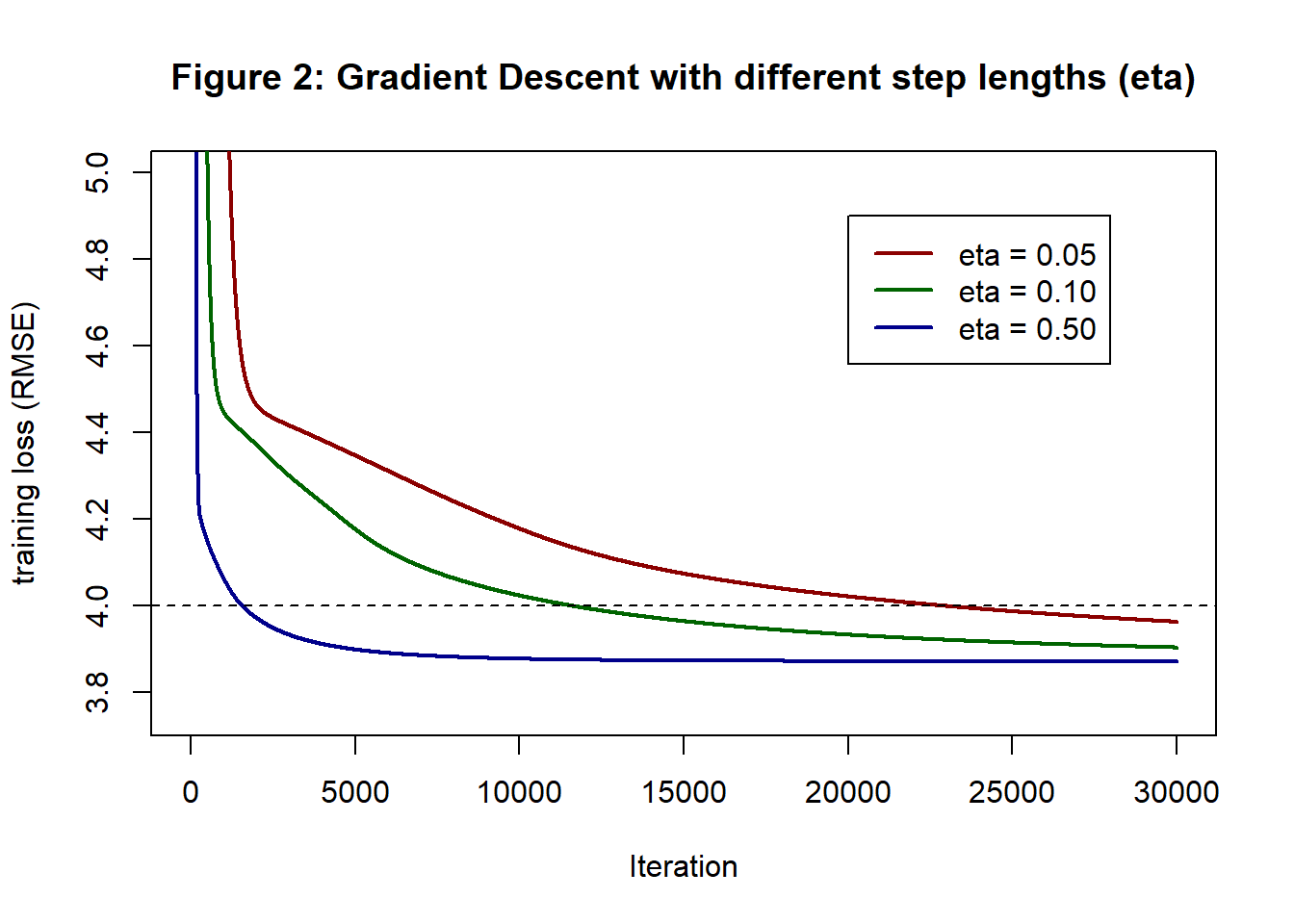
All three analyses are based on the same starting values and as you might expect, changing the step lengths makes little difference to the run times. On my home computer, the runs took 55s, 54s and 55s for 30,000 iterations. The real gain comes because with a step length of 0.5 the training loss converges after 20,000 iterations, while the other two choices would need many more than 30,000. A well-chosen step length can reduce the time to convergence by more than 50%.
With a step length of 0.5, the training RMSE at 20,000 iterations was 3.871 and this was unchanged (to 3 decimal places) at 30,000 iterations. This training loss will act as a benchmark for when we run SGD. Running 20,000 iterations will obviously be quicker with SGD, because we compute fewer gradients, but that would not be a saving if, say, it takes 60,000 SGD iterations for the training loss to drop to 3.871.
Running 20,000 iterations of GD with a step length of 0.5 took 36.6s.
Stochastic Gradient Descent.
Figure 3 shows the history of SGD run for 3,000 epochs each with 10 batch iterations, so the total number of iterations was 30,000, only now the loss is only evaluated 3,000 times. This analysis uses step length of 0.5 and a batch size of 25. The appearance is chaotic, with the algorithm jumping wildly between good solutions with low RMSEs and poor solutions with much larger RMSEs.
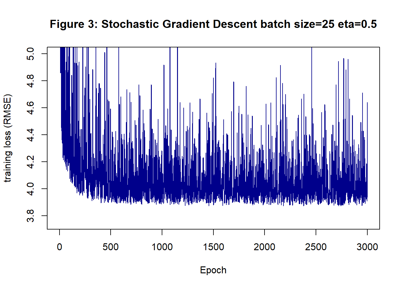
Figure 4 takes the same loss history as figure 3, but concentrates on the models with low training loss. The red curve shows the trace of the current minimum RMSE, on the left the red curve is superimposed on the chaotic history and on the right it is on its own. By 2,000 epochs the best solution has a RMSE of 3.873 and at 3,000 epochs it is 3.872; close to but not quite as good as the performance of GD. The big difference is that 3,000 epochs only took 3.3s, which is just under 10% of the time taken by GD for 20,000 iterations.
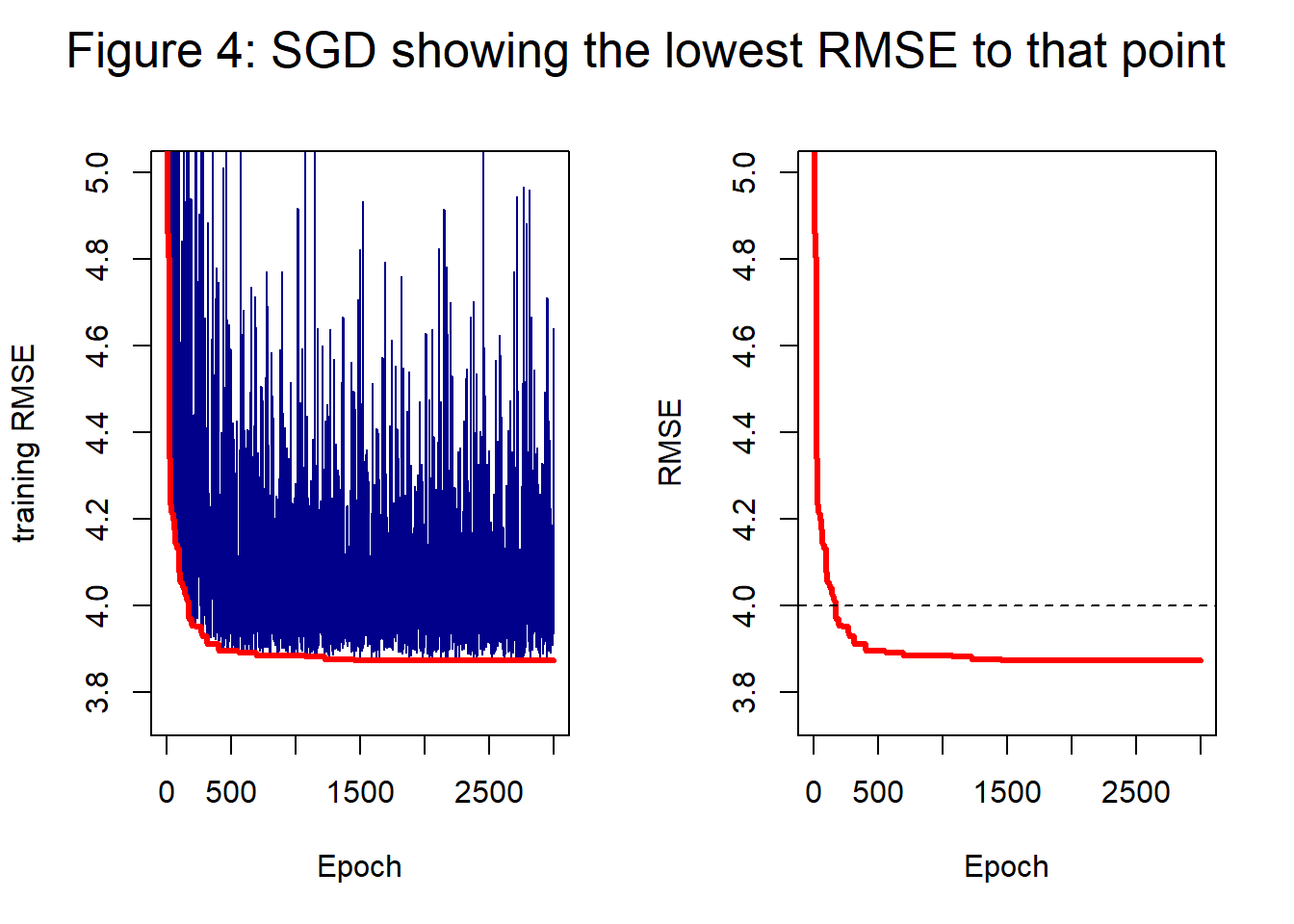
Figure 5 shows the minimum RMSE curves for SGD with different step lengths. Despite the step-like nature of these curves, they look very similar to the corresponding curves for GD shown in figure 2. It is often claimed that SGD requires smaller step sizes because of the increased danger of diverging away from the minimum when the gradient estimates are erratic. This is certainly not the case here, perhaps because the batch size of 25 gives reasonably stable gradient estimates and the model is so simple.
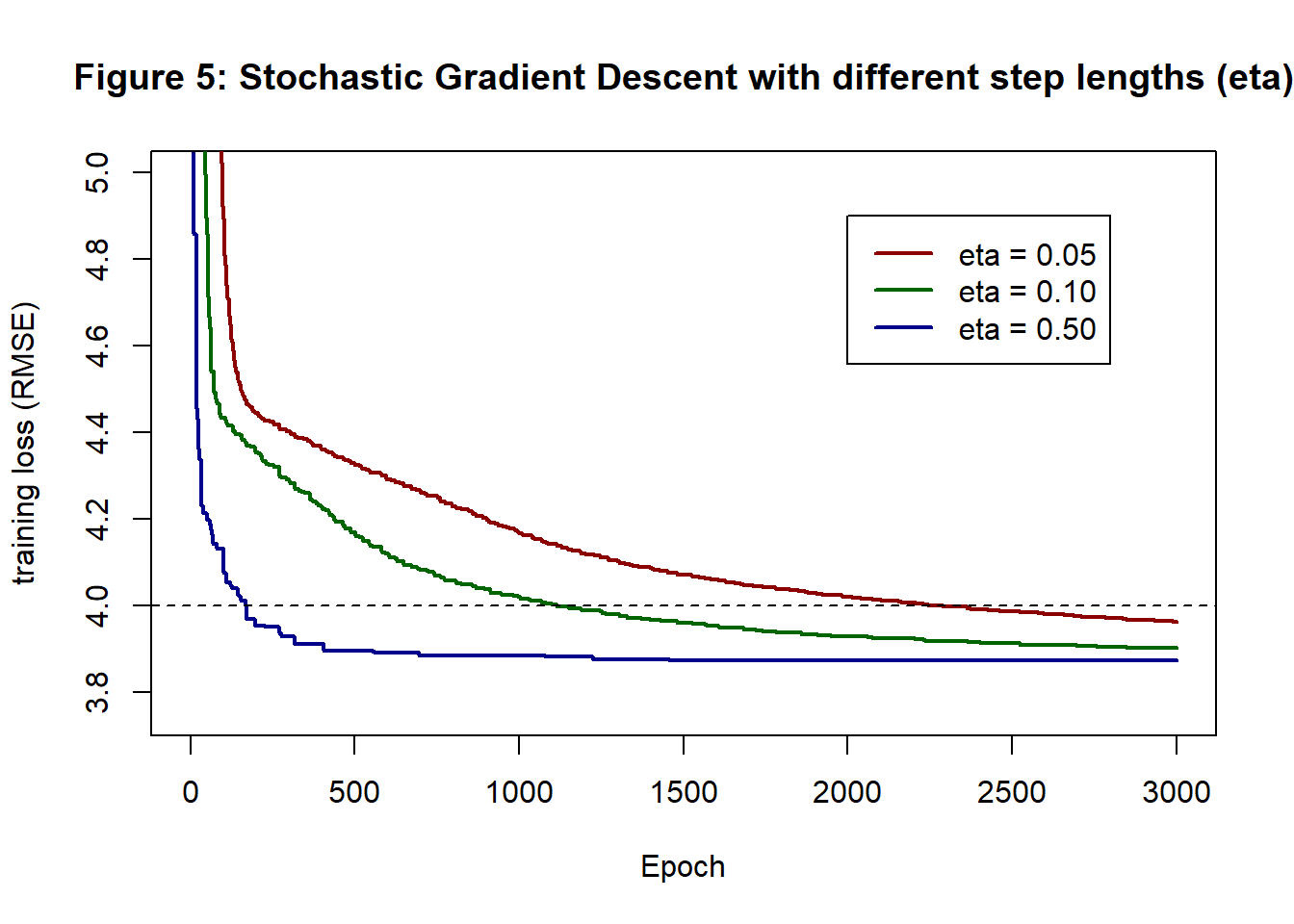
Figure 6 shows the minimum curves for a batch size of 5. Apart from being more obviously step-like, because improvements are rarer, the curves are similar to those of GD and SGD with a batch size of 25.
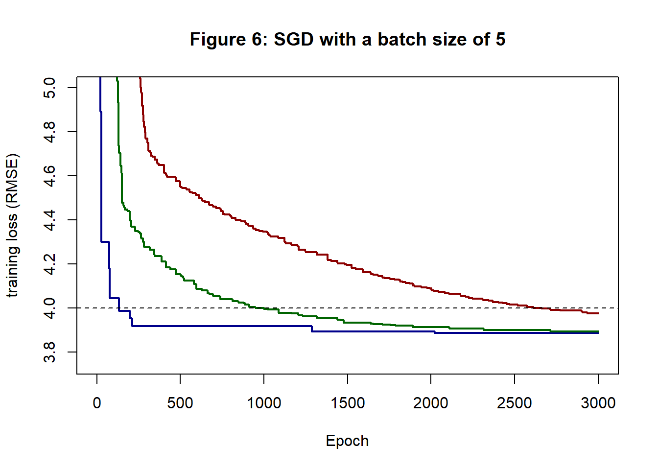
The computations with a batch size of 5 took about 2.3s, which is about 2/3 the time taken for a batch size of 25. In figure 6, the RMSE of the eta=0.5 curve at 2,000 epochs is 3.892 and at 3,000 epochs it is 3.886. Noticeably worse than GD or SGD with a batch size of 25.
A batch size of 25 takes only a little longer than a batch size of 5, but the results appear to be more dependable suggesting that it is worth the extra computation.
So what is the answer?
Look again at figure 5 and ask yourself, what model does this algorithm recommend? Were we using gradient descent the answer would be the model at iteration 30,000, or whatever run length you decide in advance is appropriate. With stochastic gradient descent the training loss is noisy and the model at epoch 3,000 (iteration 30,000) might have a low loss or a high loss, there is no way of knowing in advance.
Your choice of algorithm needs to specify in advance the method of choosing the solution. Options include
- Use the parameters (weights and biases) at the final iteration
- Use the parameters corresponding to the minimum training loss over the entire run
- Use the average parameter values over the final E epochs
- Modify the algorithm over the final E epochs so as to reduce the noise and the use the final iteration. This might be done by switching to full gradient descent.
If you have a validation sample or are using cross-validation, then there is another option
- Use the parameters corresponding to the minimum validation loss
Option 1 is unlikely to perform well because of the noise inherent in SGD and option 4 is usually impractical for all but the smallest problems. In my experience option 2 (or option 5 if there is a validation sample) works well, as does Option 3 when the parameters are averaged using exponential smoothing. I routinely use a smoothing parameter of 0.99, which makes the average depend on the last 500 or so parameter estimates.
Variations on Stochastic Gradient Descent
The hump example shows that the search path of SGD is chaotic, which may or may not be a bad thing. A chaotic search would be a problem is it failed to converge, or if it dramatically slowed down the optimisation of the training loss, but it could be a good thing if jumping between good and bad solutions allowed the algorithm to escape a local minimum and move on to a better solution.
We also need to keep in mind that our ultimate aim is to minimise the expected (test) loss and not the training loss. It is an open question as to whether the chaotic search path is more or less likely to find a solution with a low test loss? Perhaps it just increases the amount of overfitting.
There are three commonly used strategies for reducing the chaotic behaviour of SGD,
- increase the batch size
- reduce the step length as SGD approaches convergence
- smooth the derivatives by averaging them over recent iterations
Reducing the step size
For this simulation, I use a batch size of 25 and an initial step length of 0.5. Figure 7 shows the history created by my own preferred strategy of dividing the iterations or epochs into 20 blocks and reducing the step size by 10% every time the algorithm moves into a new block. The step length starts at 0.5, but by the end has been reduced to about 0.07.
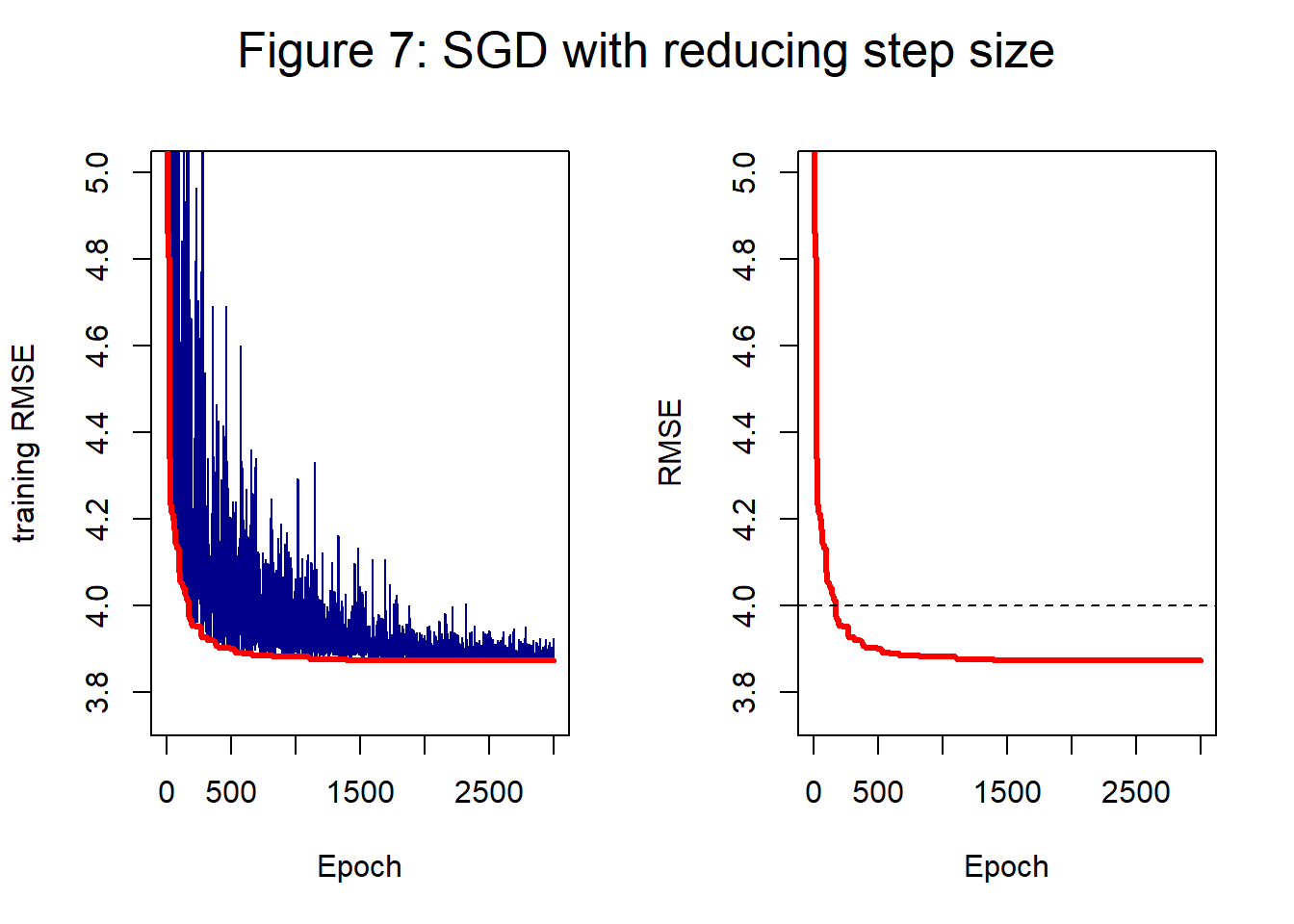
In figure 7, the training loss at 2,000 epochs is 3.873 and at 3,000 epochs it is 3.872. The chaotic behaviour is reduced but the minimum curve remains similar to that of figure 4 where the step length was fixed at 0.5.
Momentum: Smoothing the derivatives
At each iteration of the SGD, the derivatives are calculated from a fresh sample of the training data. The parameters will change very little between neighbouring iterations, so the neighbouring derivatives ought to be similar. It makes sense to average the current derivatives with those of recent iterations in order to reduce the noise. The average of the derivatives from two neighbouring iterations of SGD with batch=10 ought to have similar accuracy to the derivatives of a single iteration of SGD with batch=20.
A refinement of this idea is to use exponential smoothing in which the smoothed gradient is based on a weighted average of all past gradients with the weights declining according to the power of a chosen hyperparameter \(\gamma\), that is to say, the weights are \(\gamma\), \(\gamma^2\), \(\gamma^3\), etc. The value \(\gamma\) = 0.9 is a popular choice, that way the impact of past derivatives almost disappears after about 50 iterations.
The use of a series of powers of weights makes computation particularly simple. If we call the weighted average at iteration t, \(W_t\), and the new sample-based gradient \(G_t\) then \[ W_t = \gamma W_{t-1} + (1-\gamma) G_t \] and the parameter (weight or bias) \(\theta\) is updated according to, \[ \theta_t = \theta_{t-1} - \eta W_t \] where \(\eta\) is the step length.
Exponential smoothing requires a starting value, \(W_0\), to kick off the sequence. Conventionally, \(W_0\) is set to zero, but this choice downwardly biases the early values, \(W_1, W_2, \ldots\) A correction for this can be applied in the form \(W_t / (1 - \gamma^t)\). If \(\gamma=0.9\), then by 50 iterations \(0.9^{50} = 0.005\) and the correction makes little difference, so the effect of the starting value has all but disappeared. On the other hand, if \(\gamma=0.999\) then the sequence has a long memory and it would take over 5000 iterations for \(\gamma^t\) to get as low as 0.005. In practice, bias correction is probably not needed, but it is included in many of the papers that describe exponential smoothing of gradients and in most software.
Figure 8 shows the impact of using exponential smoothing with a parameter of 0.9; the plot should be compared with figure 4 which shows the same history without smoothing. The path in figure 8 is somewhat less chaotic, but the end result is much the same. When the loss surface is more complex or the batch size is very small, smoothing might help avoid divergence, but here it makes little difference.
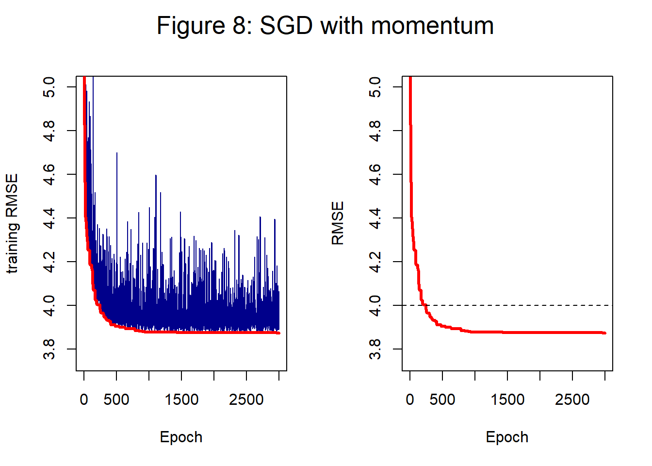
In figure 8 the training loss at 2,000 epochs is 3.875 and at 3,000 epochs it is 3.874; close to, but slightly worse, than SGD without smoothing.
As the title of this section suggests, exponential smoothing of the gradients is often referred to as momentum. The term momentum is used to convey the physical analogy of a object rolling down a hill. The direction taken is a combination of the previous directions (the object’s momentum) and the current gradient.
RMSProp
The choice of the step length is more critical for SGD than for full GD because the erratic gradient estimates create an increased risk of jumping away from the minimum. RMSProp addresses this problem of fixing the step length, but allowing it to vary automatically from parameter to parameter depending on the recent history of the SGD. RMSProp adjusts the step length of each parameter in turn so that it is reduced when the derivatives have been consistently large and increased when they have been small.
The logic is that if the gradient of a parameter has been consistently close to zero in the recent past, the algorithm must be searching a region where the loss is flat with respect to that parameter. It makes sense to try a larger step length in an attempt to escape this flat region. On the other hand, suppose that the gradient has been consistently well away from zero, the algorithm must be searching a region of rapid increase, decrease or oscillation, which argues for a smaller step length so that the algorithm does not jump over an important feature in the loss surface.
The magnitude of recent derivatives is captured by exponential smoothing of the squared derivatives. \[ V_t = \gamma V_{t-1} + (1-\gamma) G_t^2 \] The smoothing takes place separately for each parameter and update for that parameter is \[ \frac{\eta}{\sqrt{V_t}} G_t \] We can think of this as a modified step length times the gradient. A small constant may be added to the square root to avoid division by zero in flat regions of the loss surface.
An important feature of RMSProp is that when the gradient is stable \(V_t \approx G_t^2\) so \(G_t / \sqrt{V_t}\) is approximately one and the update for that parameter is \(\eta\) and not \(\eta G_t\). This means that a different initial step length may well be needed, typically a much smaller step length than for standard SGD.
A second problem occurs when the exponential smoothing is started with \(V_0=0\) as the sequence of values of \(V_t\) takes time to get away from zero. The result is that the early RMSProp updates can involve division by a number close to zero leading to early divergence. Improved behaviour can be obtained by starting with \(V_0=1\) or by running a warm-up period in which \(V_t\) is updated, but not used for the parameter updating.
Figure 9 shows the impact of RMSProp on the analysis of the hump dataset with a step length of 0.1.
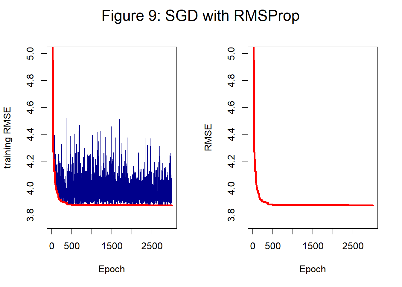
The training loss at 2,000 epochs is 3.873 and at 3,000 epochs it is 3.87. Once again the end result is very similar to that of the basic mini-batch SGD algorithm. RMSProp does not reduce the noise, but it may help convergence when the loss surface is more complex than in this simple example.
ADAM
Adam is the name given to a method proposed by Kingma and Ba in 2014. The name is taken from the leading letters of ADAptive Moment estimation. The idea is simply to use both momentum and RMSProp. The authors suggest exponential smoothing parameters 0.9 for the derivatives and 0.999 for the squared derivatives and they include the bias correction, starting the sequences at zero.
The literature is full of variations on the theme of ADAM, typically they are given names that start with ADA and they make little difference. If you look hard enough, you are sure to find a problem for which your favourite variation performs well.
Figure 10 shows the result of applying ADAM to the hump dataset. As with RMSProp it is usually necessary to have a smaller step length. Figure 10 is based on a step length of 0.1.

The training loss at 2,000 epochs is 3.874 and at 3,000 epochs it is 3.873. The history is less noisy, but the performance is not quite as good as GD.
Messy data
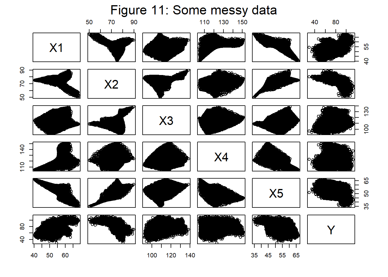
My second example consist of a training set of 10,000 observations that contains 5 predictors and 1 response. Figure 11 shows a plot of the data. They were simulated as described in my post on data - real and simulated, the random component in the response is such that a perfect model for Y would have a RMSE of 5, though of course, I will pretend that I do not know that.
Initial thoughts
The RMSE or MSE are obvious choices for the loss functions. I will adopt the robust data scaling that I recommended in my post on initial steps towards a workflow. I have no idea what neural network architecture to use, so I will start simple and try (5, 4, 1) with my favourite zero-centred sigmoid. I’ll use some variant on SGD to ease the computation; ADAM is an obvious first variation to try. Step length and number of iterations are unclear. Regularization seems to me to be unnecessary with such a simple model, but might be necessary if it turns out that I need a more complex architecture.
A key issue is how I will measure performance when I only have training data. If you have read my post on cross-validation you will know that I am not a fan. I will start by dividing the training data in two and using half for training and half as a holdout sample for validation/testing.
Step length
With my robust data scaling, step lengths between about 0.5 and 0.01 usually work well. Since there are 5 predictors my guess is that 0.5 will be too large, but I’ll try 0.5, 0.1, 0.05 and 0.01 in short runs of 1,000 epochs with 10 gradient updates in each epoch. The results are shown in figure 12.
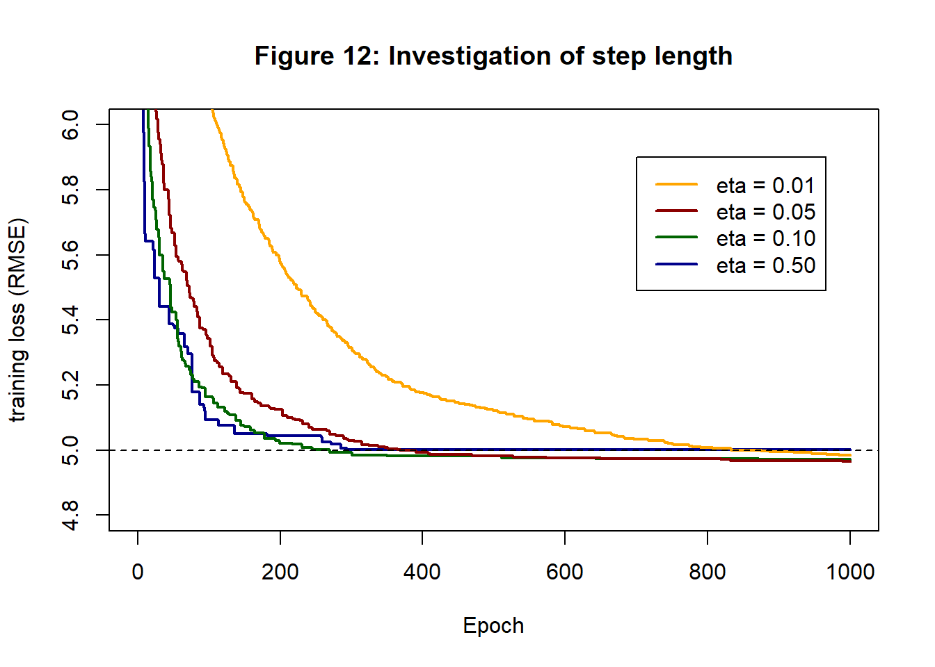
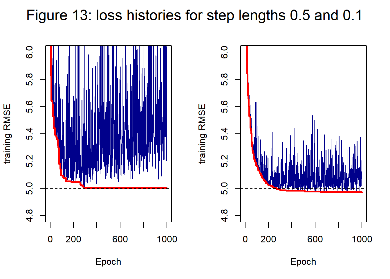
It looks as though 0.1 is best. 0.5 starts well but performance is not maintained To help further with the choice, figure 13 shows the loss histories of ADAM with step lengths 0.5 and 0.1. A step length of 0.5 leads to a more erratic history that seems to be slowly diverging after 200-300 epochs.
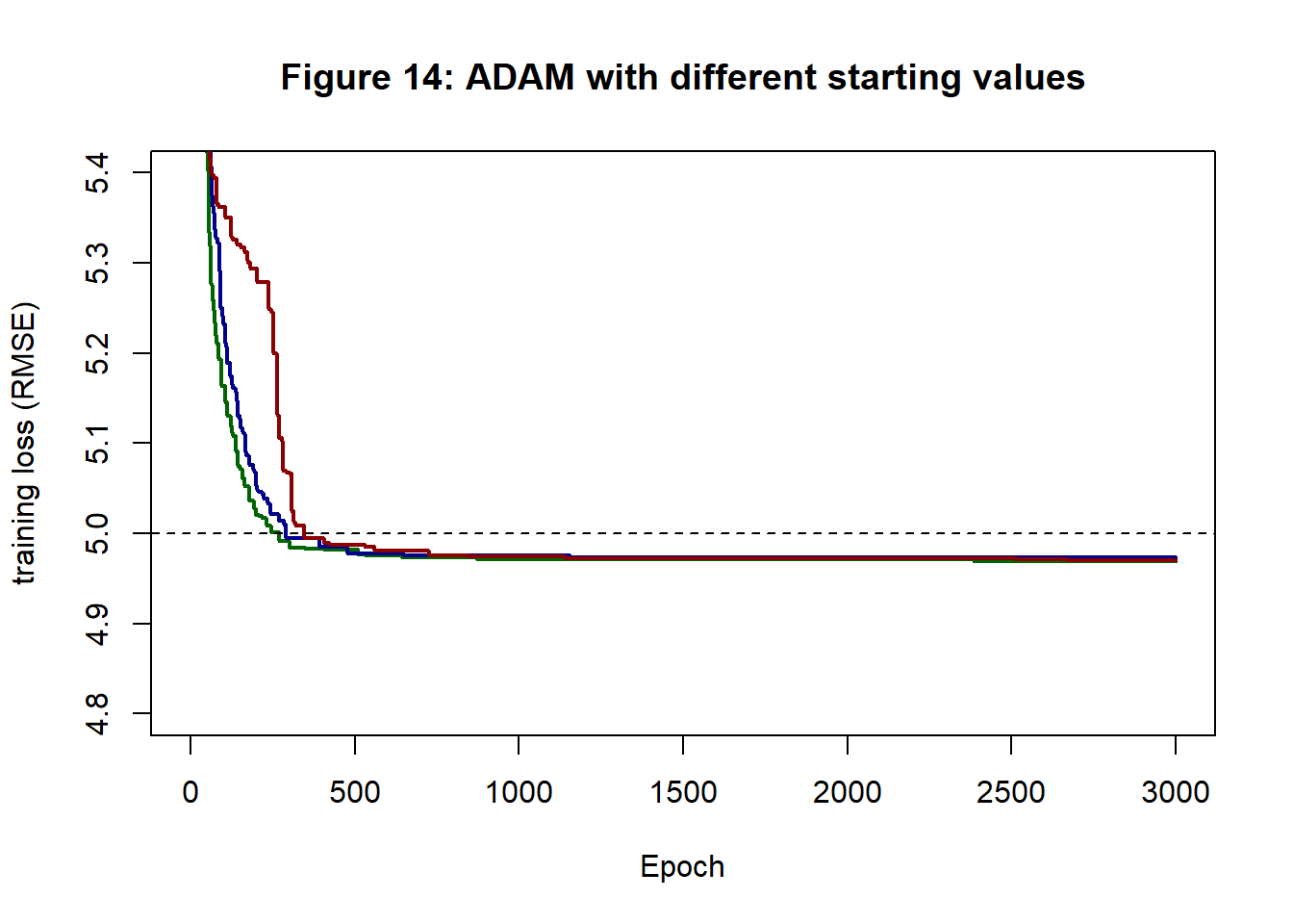
Next I tried ADAM with a fixed step length of 0.1 over 3,000 epochs. Figure 14 shows the loss histories created by using three different sets starting values. They reach very similar end points.
I modified my function cfit_valid_nn() that works for GD with a validation sample to create cStochfit_valid_nn() for SGD. In this function the validation loss is also calculated once per epoch. Figure 15 shows a plot of validation (test) loss against training loss plotted when the training loss improves; colours correspond to those of figure 14 and reflect the choice of starting values.
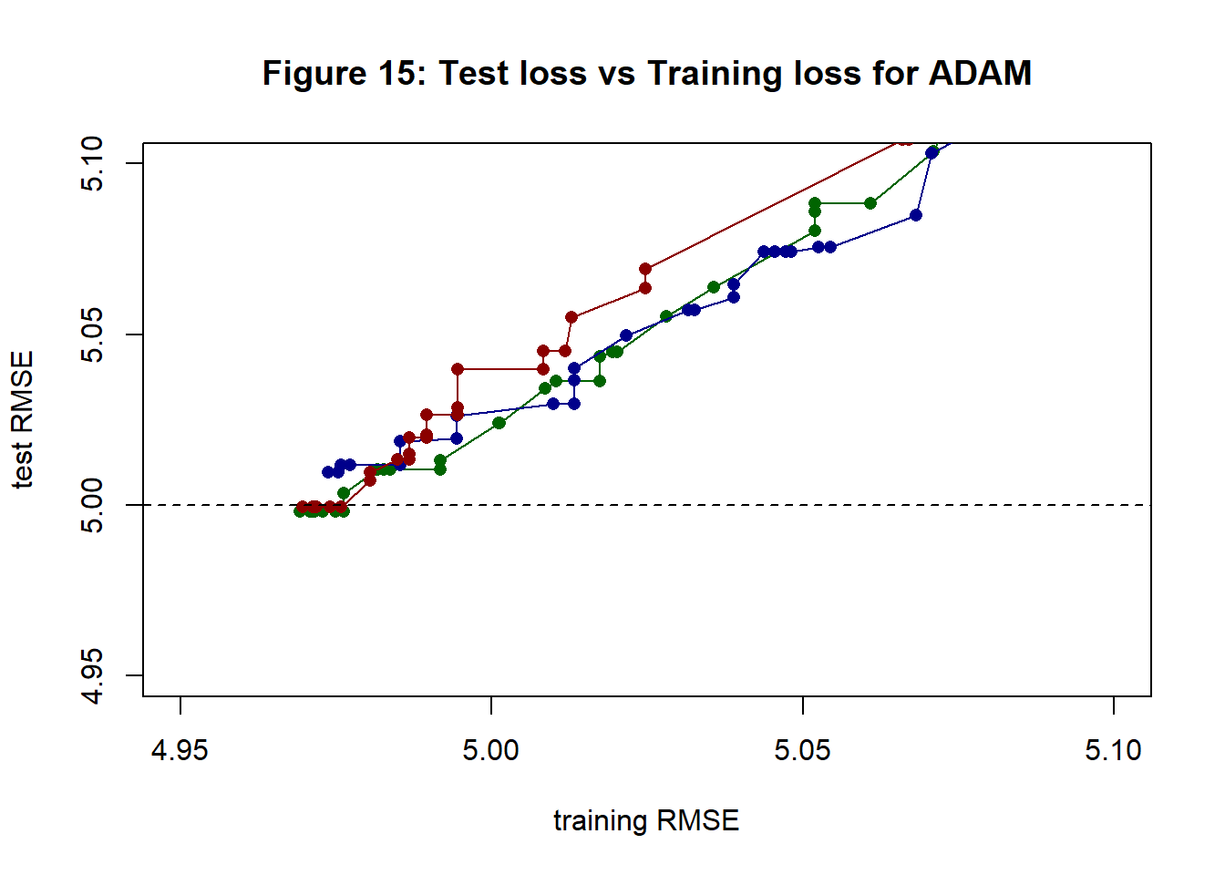
Points to note from figure 15 are,
- reducing the training loss does not necessarily reduce the test loss
- training loss becomes lower than test loss, as one would expect
- the three paths are similar
- the minimum test loss is just below 5, presumably this is a chance effect of the random split of the 10,000 observations into two halves
- there is no obvious upturn in test loss. The model only has 13 parameters and the training data has n=5,000, so one would not expect overfitting to be a big problem
- selecting a single “solution” from SGD is a bit arbitrary
In the following evaluation of the model, I use the weights and biases of the green search path at the point with minimum test (validation) RMSE. When inspecting the residuals, keep in mind that this model has been chosen for its good fit to the validation sample.
Model evaluation
There are many ways of making plots to assess model fit. I like the four part plot used by Lee, Nelder and Pawitan in their book on h-likelihood. The plot is usually based on the fitted values and residuals of the training data, but as we have a validation set Figure 16 uses the validation fitted values and residuals (it makes almost no difference).
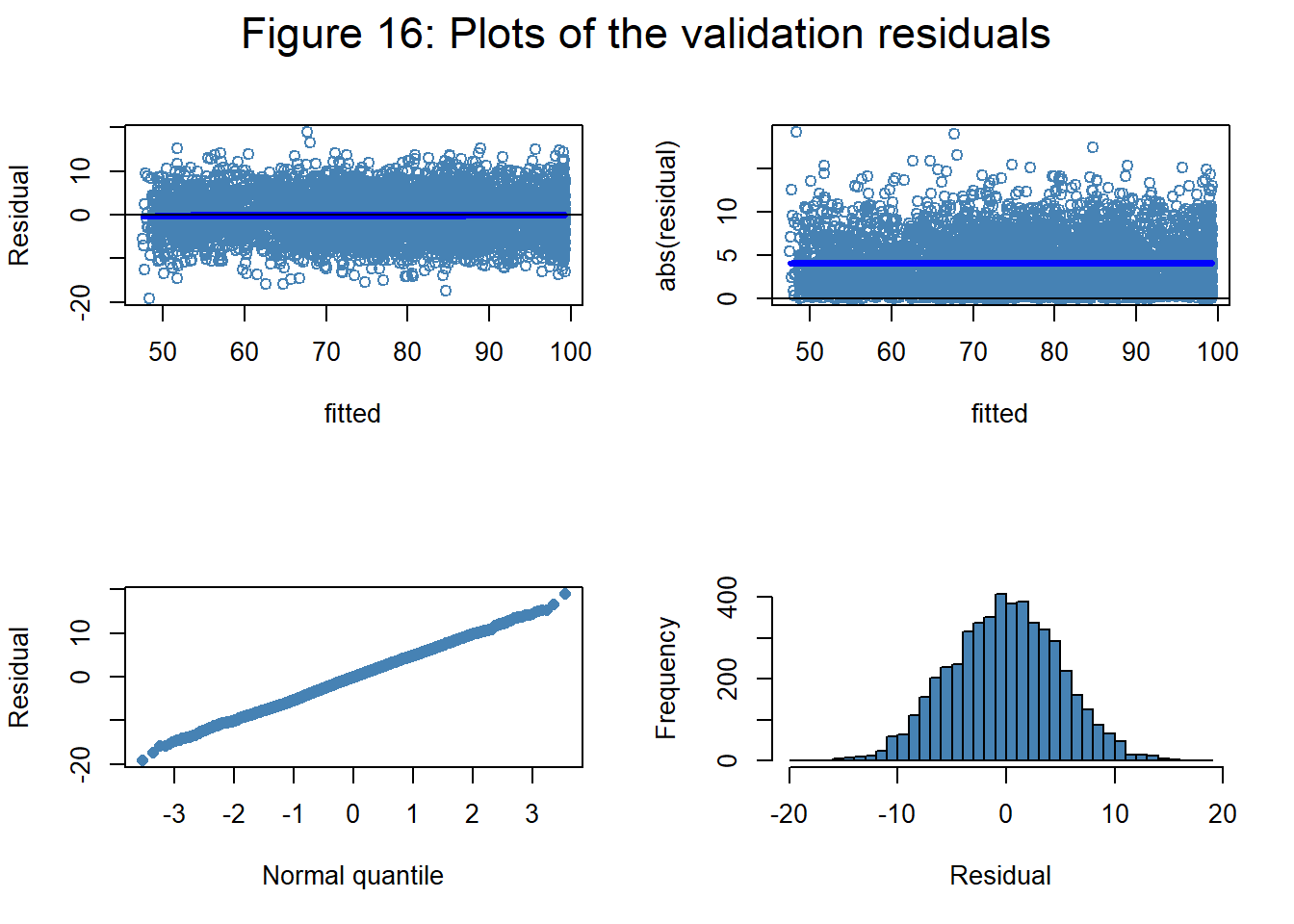
The top left shows the plot of residuals against fitted values together with a loess smooth shown in bright blue. When the loess smooth is not a horizontal line, it indicates that the model has missed an important component of the trend. In this case, the model has done a good job. The second plot shows the absolute residuals against the fitted values. This plot helps detect regions of high or low variance. These data were simulated with constant variance and that is confirmed by the plot as the loess smooth is a horizontal line. The third plot shows the ordered residuals against Gaussian quantiles; a straight line indicates normality. The simulation did indeed use Gaussian noise and, reassuringly, the points do lie close to a straight line. Finally, there is a histogram of the residuals confirming normality with a mean close to zero and a standard deviation close to 5.
The neural network seems to have done a very good job of modelling the data.
Examining the fit
Judged by the second panel on the bottom row of figure 11, X2 will be an important predictor of the response, so I use it to illustrate my plot of the marginal fits. I divide the range of X2 in the validation sample into bands, in this case of width 2 and then I find the mean response Y within each band and the 80% interval for the data. In Figure 17, these are shown in red; they act as a summary of the pattern in the validation data and should correspond closely to the pattern seen in the second panel of the bottom row of figure 11. On top of these red observed intervals, I show in blue the average predicted response for observations that fall in that band; these predictions are based on the fitted model, the validation sample and all of the predictors.
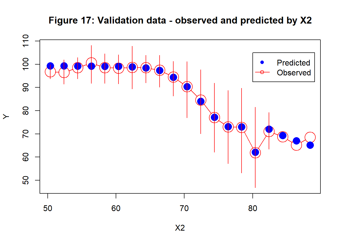
Figure 17 shows how the response changes with X2 and how the model does a very good job of capturing that trend. Perhaps the model slightly over-estimates the response in the first few bands and under-estimates with the highest X2, but these are the bands with the fewest observations.
The corresponding plots for the other 4 predictors are shown in figure 18.
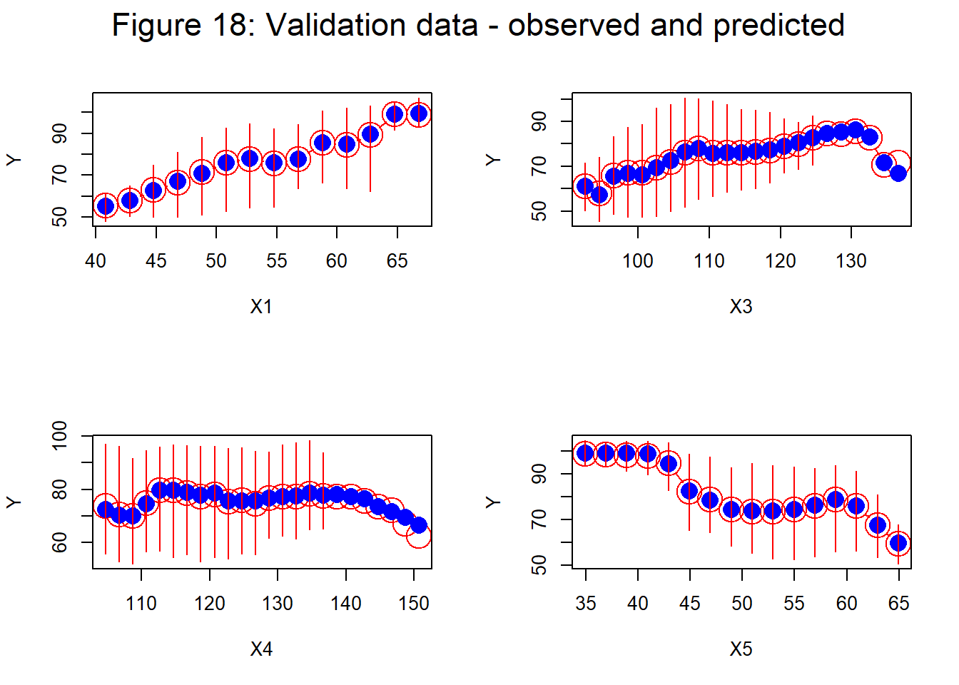
Agreement between average observed and predicted values is again very good. The only slight disagreements are seen close to the ends of the ranges. Bands with no 80% range reflect sparseness of the data within that band.
Despite the non-linearities and mild interactions of my simulated data, the underlying trend is found with remarkable accuracy by a (5, 4, 1) neural network and I do not feel the need to try anything more elaborate.
Conclusions
Here are the points that I take from this post.
- SGD works well with very small batch sizes, but the path can be noisy
- even in my simple examples, the saving in computation time of SGD is quite dramatic. The gain would be much greater for larger training sets or more complex models
- it is important to find an appropriate step length before you start SGD
- momentum reduces the noise, but does not improve the speed of convergence
- RMSProp gives more reliable convergence, but does not decrease the noise
- ADAM is a good general purpose algorithm
- there is an issue over what you take as the solution from SGD, given that the last iteration may not have a low training loss. Exponential smoothing over the final iterations is a good option.
Appendix: Code Changes
The C code used in this post can be found on my GitHub pages as cnnUpdate04.cpp.
I added functions to cStochfit_nn() and cStochfit_valid_nn() that enable stochastic gradient descent with a user specified batch size. Options momentum and rmsprop add those variations. To replicate ADAM use both momentum and rmsprop.
In cStochfit_valid_nn() the validation loss is only calculated when the algorithm finds a new lowest training loss.
Appendix: References
Lee, Y., Nelder, J. A., & Pawitan, Y. (2018). Generalized linear models with random effects: unified analysis via H-likelihood (Vol. 153). CRC Press.
Kingma, D. P., & Ba, J. (2014). Adam: A method for stochastic optimization. arXiv preprint arXiv:1412.6980.