Neural Networks: Regularisation and overfitting
Introduction
In this series of posts, I am trying to discover how best to use neural networks on tabular data by experimenting with small simulated datasets. So far, I have
- written R code for fitting a neural network by gradient descent
- used Rcpp to convert the R code to C for increased speed
- pictured gradient descent search paths
- used neural networks to simulate datasets for use in my experiments
- made some tentative first steps towards a workflow
- considered the pros and cons of cross-validation
- extended the workflow to include classification problems
This time I investigate two related topics that are fundamental to machine learning, but which are usually treated in a hand-wavy way, namely overfitting and regularisation.
What exactly is regularisation?
When I started to read the literature on machine learning, the concept that caused me the most difficulty was regularisation. It is not that the ideas were new to me, they are all well-established in statistics, it is more that in machine learning the term seems to change its meaning to suit the needs of the author. As with so many concepts in machine learning, regularisation is assumed rather than defined.
I suspect that the root cause of the lack of clarity is that the term regularisation is used to refer to three distinct issues relating to the minimisation of the training loss of a flexible model.
- a model with a very low training loss, often predicts poorly on new data
- the minimisation is often be ill-posed, so that there are many equivalent solutions, i.e. there can be very different models with the same low training loss
- standard loss functions depend on the difference between a measured response and a predicted response, they make no adjustment for the complexity of the model that produces the prediction
The first of these issues is sometimes called overfitting. So, for some people, regularisation is anything that reduces overfitting. Of course, this begs the question, what exactly is overfitting?
The second issue relates to the efficiency of the algorithm. When there are many equivalent solutions, the algorithm may travel between them and find it difficult to settle on any one.
The third issue is perhaps the most challenging. Occam’s razor, says that when you have two competing explanations, prefer the simpler. I think that most data analysts would be happy to extend this idea and say that, if you have two competing models that predict equally well, prefer the simpler. There is less to go wrong with a simple model and when something does go wrong, it is easier to spot. Unfortunately, this leaves us with an even more difficult question, how do you measure model complexity?
Overfitting
Five Challenging Questions
The machine learning literature is just as vague about overfitting as it is about regularisation. Everyone knows what it means (in a hand-wavy way), so why define it?
You probably already have a general idea of what overfitting is, so let’s test your understanding with these five questions.
- Is overfitting a property of an algorithm or a property of a model?
- If the training data change, will that affect whether a model/algorithm overfits?
- Is the training loss of an overfitting model/algorithm always lower than its expected (test) loss?
- If the test loss along an algorithm’s search path starts to increase, is the model/algorithm overfitting?
- Does a model/algorithm overfit if there is an alternative model/algorithm with fewer parameters that has the same training loss?
Here are my answers to these questions. They summarise an opinion, so you might not agree.
- Overfitting is a property of the model and not the algorithm. How you come up with that model is irrelevant to whether or not it overfits
- Yes, changing the data affects overfitting. Overfitting depends on both the model and the training data
- Probably, but not in every case, as I will show shortly
- Overfitting is not a property of the algorithm, so the search path is irrelevant.
- No, this question refers to model complexity not overfitting. Incidentally, the number of parameters is a poor measure of model complexity.
One Challenging Example
Figure 1 is designed to challenge your concept of overfitting. It shows two models fitted to the same red training data, one model is in blue and the other is in green. The question is, which of the models overfits?
In the figure, the training data vary randomly about the points where the curves cross. So, as the red line shows, the distance between the training value and the prediction according to the green curve is also the distance between the training value and the prediction of the blue curve. Judged by any reasonable loss function, the two models are equally close to the training data, i.e. they have exactly the same training loss.
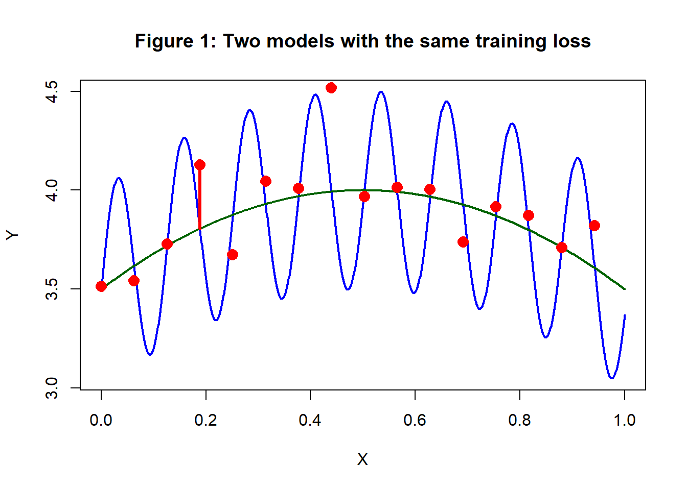
Not unreasonably, you probably think that the blue curve in figure 1 is overfitting, but perhaps the test data wiggle like the blue curve and the green curve underfits. Belief that it is the blue curve that overfits comes not from these data, but from your experience of data analysis; the green pattern is much more common and of course, it has the advantage of being simpler.
My definition of overfitting
Having criticised the machine learning literature for its vagueness, I have no option but to describe my own understanding of overfitting, regularisation and model complexity. I’ll start with overfitting, knowing that this will not be easy and that any definition that I propose will have its own weaknesses and it will probably irritate some people, but at least I am going to try.
A Diagram showing overfitting
I will base my definition on a plot of expected loss against training loss of the type that I introduced in my earlier post on search paths. It is meant to be a diagrammatic representation, not an exact plot.
Every model with fully specified parameter values has an expected loss and a training loss, so it can be plotted as a point in the diagram. It is possible that two different models, e.g. neural networks with different weights and biases, might have the same losses and so be represented by the same point.
Figure 2 shows the model space for a particular analysis by the red parabolic shape, perhaps it might include all possible (4, 5, 2) neural networks. The best possible model within the chosen family is the one with the lowest expected loss and it is represented by a red dot.
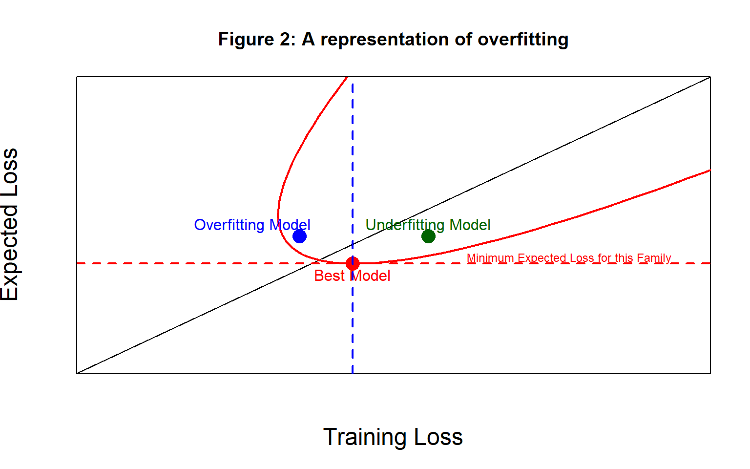
Here is my definition,
a model overfits if it has a training loss that is smaller than the training loss of the best model in the family and it underfits if its training loss is larger than that of the best model
In the diagram, the blue dot represents an example of an overfitting model and the green dot represents a model that underfits.
Notice that I have deliberately chosen to define overfitting without reference to the model’s expected loss. If you don’t like my approach, this choice is probably at the heart of our disagreement. The diagonal line shows equality between the expected loss and the training loss, so an overfitting model can have a training loss that is larger than the expected loss (below the line of equality) or it can be smaller (above the line).
In figure 2, the overfitting model is less than ideal (i.e. its expected loss is above the minimum), because it has started to follow the noise in the training data, while the underfitting model is less than idea because it has not adequately captured the trend common to all data from that source. Importantly, I have chosen my examples of overfitting and underfitting models to have exactly the same expected loss. This means that their predictive performance will be the same. It is not overfitting that you want to avoid, rather you want to avoid models with a large expected loss.
Let me acknowledge a limitation of my definition. In practice, we will not know the form of the best model in the family, so we will not know its training loss and we will not be able to test for overfitting. I’ll return to this issue shortly.
Overfitting and an algorithm’s search path
When we fit a neural network to a set of training data by gradient descent, we chose random starting values and then improve the training loss in small steps. These steps correspond to movements to the left in my diagram. Unless you employ an early stopping rule, the algorithm will stop when it either reaches a local minimum of the training loss, or when it finds the global minimum.
In figure 3, the path taken by the algorithm is shown as a brown dotted line and the point along the path with the minimum expected loss is the model that you would ideally likely to choose and it is shown as a dark green dot. I’ll refer to it as the best fitted model. It so happens that for this algorithm and these starting values, the best fitted model underfits the data.
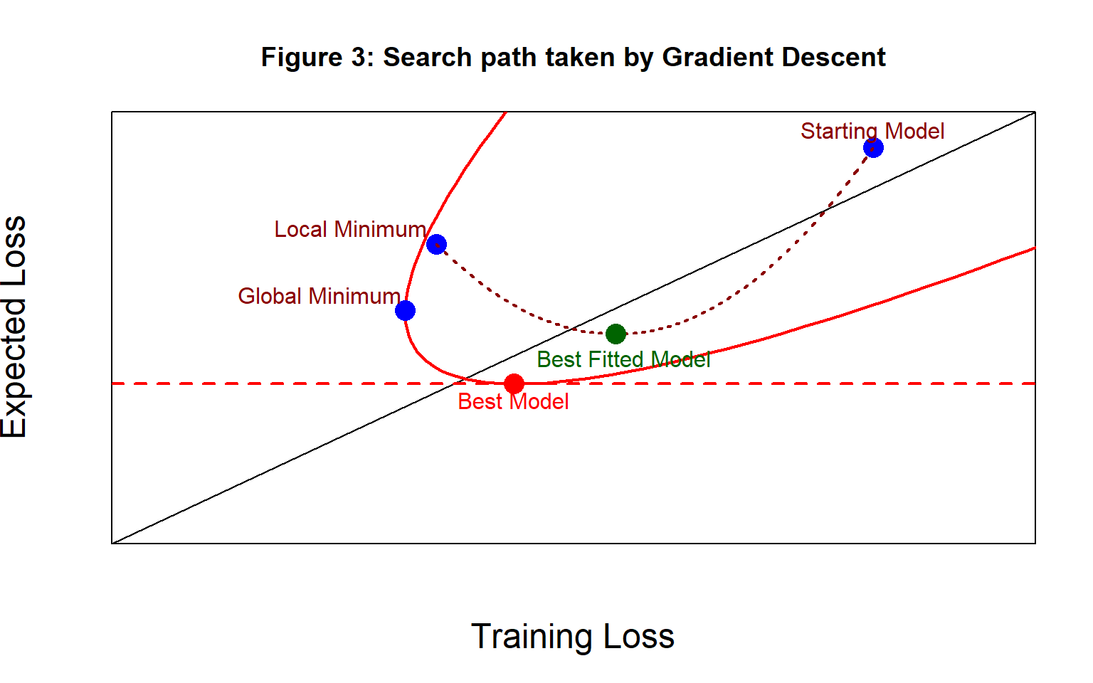
Having visited the model with the minimum expected loss, the algorithm continues to reduce the training loss, but the expected loss increases. For a while, the models on the search path in figure 3 continue to underfit the data, but by the time that the algorithm converges to a local minimum, the models are overfitting.
Clearly, you could have a combination of algorithm and starting values for which the algorithm only ever visits underfitting models, or a combination that only ever visits overfitting models.
Maybe you have run many different algorithms from different starting values and you believe that the best of all of your chosen models is close to the best possible model for that family. In these circumstances, you could use the training loss of the best fitted model as an approximate threshold for judging overfitting.
Regularisation
Because regularisation relates to overfitting, ill-posed minimisation and model complexity, I am reluctant to define it in terms of overfitting alone. Instead, my definition is,
regularisation is the use of external information to restrict the model space
By external information, I mean anything other than the training data. Examples relevant to a⌈ neural network include,
- you believe that the weights of the fitted model will be under 5 in magnitude
- you believe that the fitted curve will not be as wavy as the blue curve in figure 1
- you believe that a high proportion of the weights will be zero
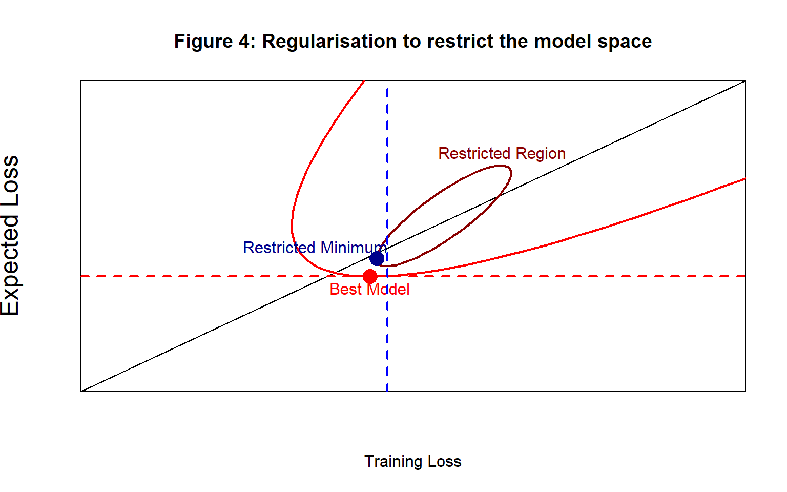
Figure 4 shows a diagrammatic representation of a restriction of the model space. The algorithm is limited to considering models within the brown ellipse. Clearly, it is possible to impose restrictions that concentrate the search close to the Best Model, or to choose the restrictions poorly and pull the search away from the Best model. It all depends on the quality of the external information.
Unlike overfitting, which is a property of a model, regularisation is a constraint on the algorithm.
Bear in mind that restrictions are rarely as absolute as the one shown in figure 4 where models outside the brown ellipse are ruled out entirely. It is much more common to apply some form of weighting, so that particular models are not ruled out, but instead they become less likely to be visited by the algorithm.
Ill-posed minimisation
The simplest regression neural network has one input X, one hidden node and one output, \(\mu\), that predicts the response Y. Such a neural network is shown belowIn this picture the input, X, is multiplied by the weight \(w_1\), the bias \(b_1\) is added and then the combination is passed through an activation function \(\sigma()\). The result A is multiplied by weight \(w_2\) and bias \(b_2\) is added to get the prediction, \(\mu\).
With a sigmoid activation function, the central part of the sigmoid curve is almost linear with a slope of 1/4, so provided we stay within that region the prediction will take the form \[ \mu \approx w_2 \frac{w_1 \ X + b_1}{4} + b_2 = \frac{w_2 \ w_1 \ \ X}{4} + \frac{4 b_2 + w_2 \ b_1}{4} \]
If the true relationship is, say, 2X+1 then we just need to make \(w_2 w_1 = 8\) and \(w_2 b_1 + 4b_2 = 4\). There are no end of possible solutions; \(w_2\)=1, \(w_1\)=8, \(b_1\)=1, \(b_2\)=0 or \(w_2\)=2, \(w_1\)=4, \(b_1\)=1, \(b_2\)=-1/4 etc. etc.
Set an algorithm to estimate the weights and biases and there will be a danger of it flipping forever between equivalent solutions and even if it does settle, there is no knowing which solution the algorithm choose. Of course, there is a sense in which it does not matter which solution you get; they may look different, but their predictions will be the same.
The real problem is the difficulty that an algorithm has in settling on one solution when there are so many to choose from. To make matters worse, these solutions are not discrete and well separated. If \(w_2\)=1, \(w_1\)=8 is a solution, then so is \(w_2\)=1.001, \(w_2\)=7.992; the solutions form long flat bottomed gorges through the loss surface. The algorithm may find it easy to drop into a gorge, but then it will move backwards and forwards along the bottom without ever finding a unique solution.
Larger neural networks have a second problem, they have many symmetries. Take a (1, 2, 1) algorithm as a simple example and swap the weights and biases between the two hidden nodes; the predictions will be unchanged. Symmetries are usually less of a problem, because the equivalent solutions are likely to be well separated in the space of the parameters and although we cannot tell which solution the algorithm will settle on, at least it is unlikely to flip from one to another.
To overcome these problems and make the solution unique, we need to supply the algorithm with external information that ranks the many possible solutions. This information will be external to the training data and it will restrict the model space, i.e. it will regularise the algorithm.
Model complexity
Let’s return to the example shown in figure 1 with its blue and green curves that have exactly the same training loss and suppose that the green curve is close to the truth, that is, it a good approximation to the best model in the family. Figure 5 represents the two models with their equivalent training losses. The assumption here is that we are using a neural network architecture that is complex enough to capture both curves, perhaps we played safe and used the (1, 20, 20, 1) family of neural networks.
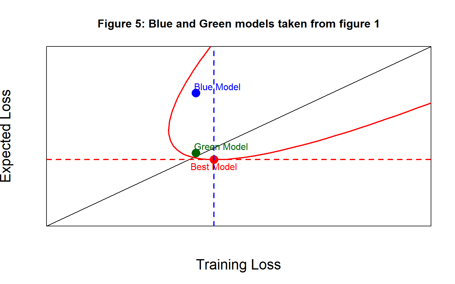
Both models have the same training loss, but the blue model would predict poorly with new data and so has a much larger expected loss. As I have drawn it, both models slightly overfit this particular set of training data (by my definition).
An algorithm that seeks to minimise the training loss would have no reason to prefer the green model over the blue model. Preference for the green model is based on external information. The way to ensure that the algorithm picks the green curve is to restrict the model space perhaps by,
- down-weighting wavy models i.e. models with large second derivatives
- down-weighting complex models
In this context, what is meant by a complex model? Both curves are based on the same neural network architecture, so they have access to the same number of parameters. The difference is that to get the shape of the blue curve you will need to use all available weights and biases, but you could get the green curve or something very close to it, even if you set many of the weights and biases to zero i.e. the green curve does not need such a complex architecture.
In this case, we could get the algorithm to favour the simpler solution by placing a restriction on the model space that encourages zero weights and biases. The justification for this restriction would be a belief that the truth will be simple, this belief is external to the data, so it would be the basis of a form of regularisation.
The research literature is full of suggestions of ways to measure complexity, but most of them are themselves complex and they would be difficult to use within a search algorithm. In contrast, encouraging zero weights turns out to be simple to implement, as we will see shortly.
Types of regularisation
The classic way to regularise is to add a penalty term to the loss function that down-weights some models and encourages others. In my opinion, this is the best method, because it is explicit, which means that you can see clearly which models are favoured and other people can judge whether your chosen regularisation is sensible. Remember, regularisation uses external information and so, it almost always involves an element of subjectivity.
Penalty terms that depend explicitly on the parameters are particularly easy to use in gradient descent as the derivative of the penalty with respect to each parameter is simply added to the derivative of the basic loss.
Some machine learning techniques regularise as a by-product; this is sometimes called implicit regularisation. A good example of this is early stopping. You might believe that if you run gradient descent to convergence of the training loss, you will eventually visit models that overfit. Loosely speaking, you imagine the models becoming too wavy as they capture random fluctuations in the training data. Stopping before convergence will shorten the search path and avoid such models.
The external information in early stopping comes from your knowledge about the way that the gradient descent algorithm works. The weakness of this approach is its indirectness. It is hard to justify one early stopping rule over another and it is difficult to relate a chosen rule to the set of models that are avoided.
Other methods of implicit regularisation. That is to say, methods that have regularisation as a side-effect include,
- data augmentation, artificially manufacturing more training data
- averaging over multiple models
- drop-out (randomly dropping nodes from a neural network)
- model simplification/pruning/selection
Implicit regularisation is often easy to implement, but difficult to control. In my opinion, it is far better to impose restrictions in an explicit way.
Explicit Regularisation with a Prior
Suppose that I want to regularize a neural network by down-weighting very large weights and biases. I’ll refer to the biases in my explanation, but the same argument would apply to the weights.
Suppose that I take the view that biases are unlikely to be over 5 in magnitude, larger biases would force the linear predictor into the tails of a sigmoid activation function, where all inputs would be converted to more or less the same output. However, I am reluctant to rule out larger biases completely; after all, unexpected things do happen. In a Bayesian analysis, I might quantify this belief by placing a Gaussian prior on each of the biases, \(\beta_i\), say, \[ \beta_i \sim \text{N}(0, \text{sd}=\sigma_\beta) \ \ \ \ i=1,\dots,m \] with \(\sigma_\beta\) equal to say, 2 or 2.5.
In a neural network the parameters are estimated my minimising a loss function that is typically chosen to have the form of minus twice a log-likelihood to which minus twice the log of the Gaussian prior would be added to obtain something within an additive constant of the log posterior. Assuming that you have no preference for positive biases over negative biases, the component of minus twice the log of the Gaussian prior that depends on \(\beta\) is, \[ \frac{1}{\sigma_\beta^2}\sum_{i=1}^m \beta_i^2 \]
If you are uncomfortable with assigning a value to \(\sigma_\beta\), then you might write the penalty as \[ \lambda\sum_{i=1}^m \beta_i^2 \] and then the value of \(\lambda\) could be determined by hyperparameter tuning, perhaps by using cross-validation. This function is often referred to as the L2 penalty.
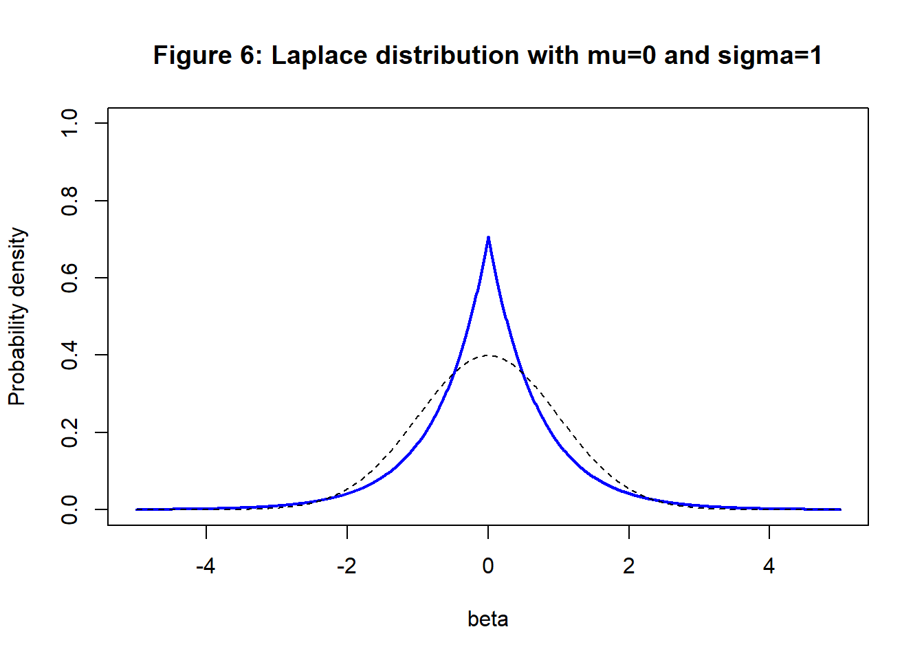
In much the same way, a Laplace prior leads to the L1 penalty, \[ \lambda\sum_{i=1}^m |\beta_i| \] The Laplace prior has the form \[ p(\beta) = \frac{1}{\sqrt{2} \sigma_\beta} exp \left\{ -\frac{\sqrt{2}| \beta - \mu_\beta |}{\sigma_\beta} \right\} \] This distribution has longer tails and is shown in figure 2. A Laplace(0, \(\sigma_\beta\)) prior is appropriate if you believe that most of the biases will be close to zero with a few large biases. In figure 2 a standard normal distribution is shown as a dashed line for comparison.
A uniform prior, say U(-5, 5), is flat so it treats all biases in this range as equally likely. The penalty is a constant and does not affect the minimisation of the loss. However, biases outside (-5, 5) are deemed impossible, so the loss would be minimised over the restricted range.
Selecting lambda
In the C code available on my GitHub pages, the loss and its derivatives for flexible regression models are based on the sum of squared errors, although the mean square error is returned as the lossHistory. On this scale, the value of lambda is the ratio of the variance of the training data about the model and the variance of the prior on the model parameters, i.e. \(\lambda=\sigma_y^2/\sigma_\beta^2\).
An approximate value for \(\sigma_y\) can be obtained by running the gradient descent algorithm without any penalty and using the root mean square error or even by running linear regression on the features. \(\sigma_\beta\) expresses your personal belief about the sizes of the parameters. If you are unsure as to the magnitude of the parameters, then you could make this value very large, in which case \(\lambda\) will be close to zero and the penalisation would have very little impact. Making \(\sigma_\beta\) large will not force the parameters to be large, the analysis learns about the parameters from the training data, all that large \(\sigma_\beta\) says is that you have no external information to make you prefer small parameters over large ones. In contrast, a small value for \(\sigma_\beta\) (large \(\lambda\)) means that you have reason to expect the parameters to be close to zero, this will have the effect of restricting the algorithm to parameters that are smaller than the data alone would suggest. Reducing the size of the parameters will tend to make the model smoother and less wavy.
It is my practice to scale the response variable so that most of its values lie in the interval (-5, 5). This corresponds to the interval in which I would probably expect the biases to lie. Consequently, in problems where the features are poor predictors, with my C code \(\lambda=1\) is often a good choice for the penalty. If the model explains half of the variance then \(\lambda=0.5\) would be a better guess.
Some data scientists rely heavily on hyperparameter tuning. Essentially, they try many different values of \(\lambda\) and select the best according to some criterion, usually based on cross-validation. I am not keen on hyperparameter tuning. The variance in cross-validation and related methods is usually so large that picking the best value for the hyperparameter is akin to buying a lottery ticket, so hyperparameter tuning gives a false sense of security. In my experience, small differences in lambda make very little difference to the final model and meaningful differences in lambda can be judged subjectively.
The wave
In some of my earlier posts, I have analysed simulated data with a pattern that I call a wave. The generating curve and a set of 100 training values is shown in figure 7.
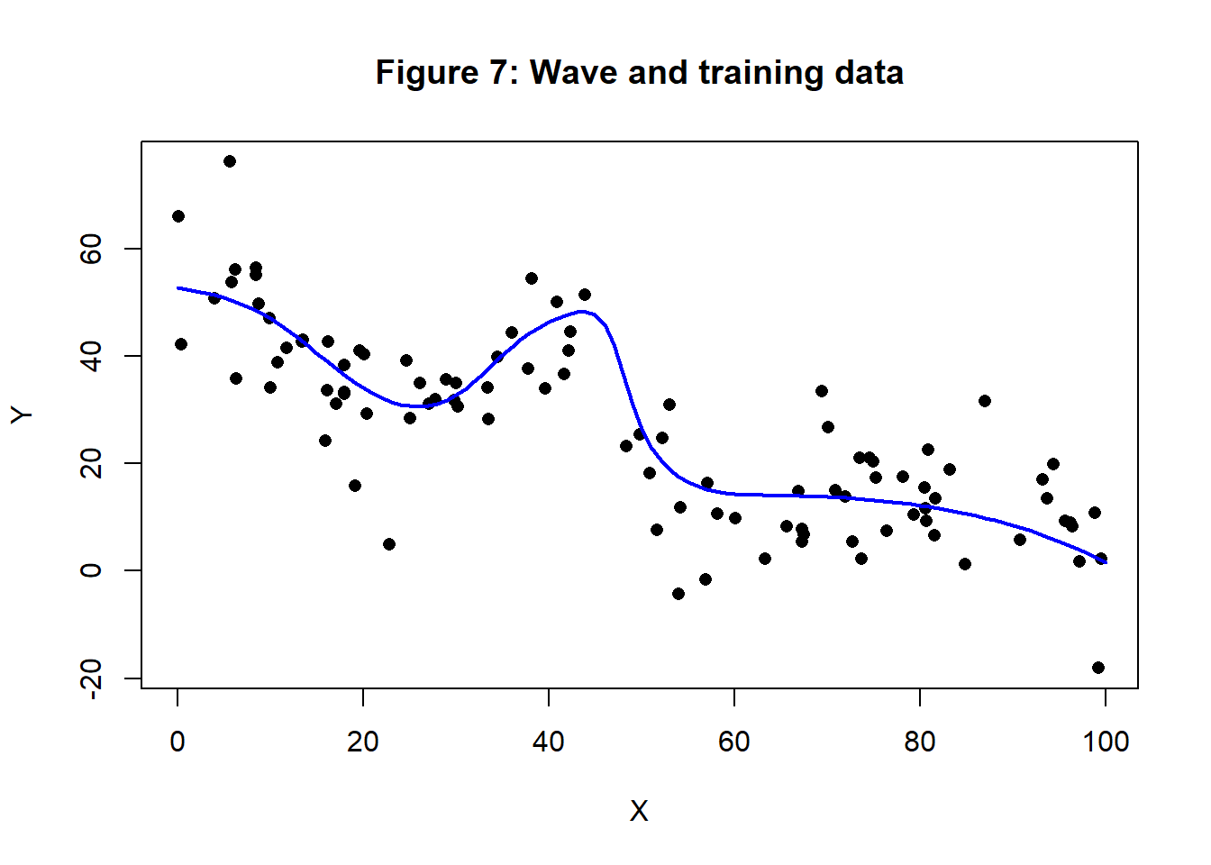
Figure 8 shows the history of the MSE of a gradient descent algorithm with robustly scaled data and no regularisation penalty when it is used to fit a (1, 8, 1) neural network to these training data.
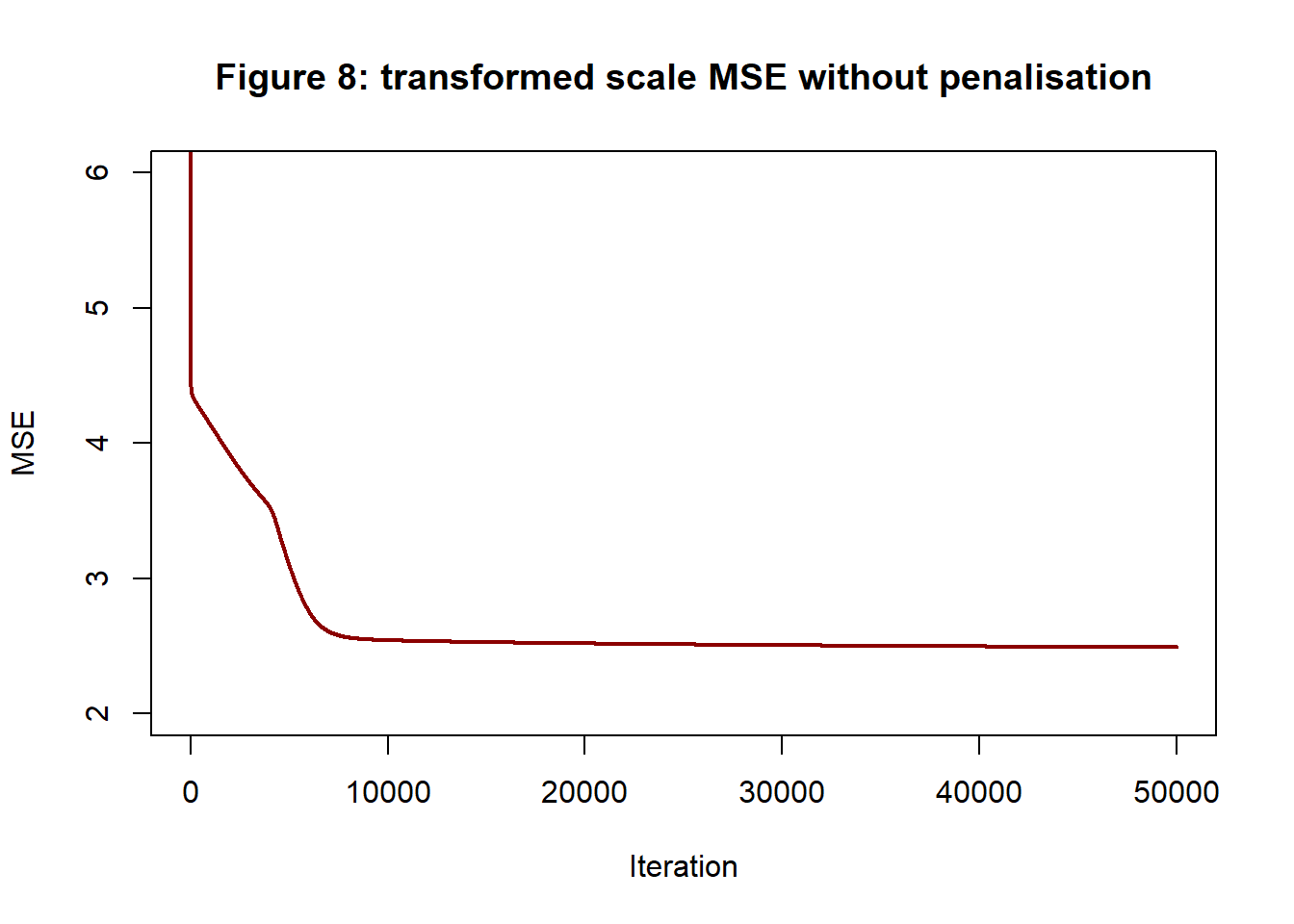
So the MSE of the fitted model is about 2.5.
Figure 9 shows the fitted model superimposed on the training data
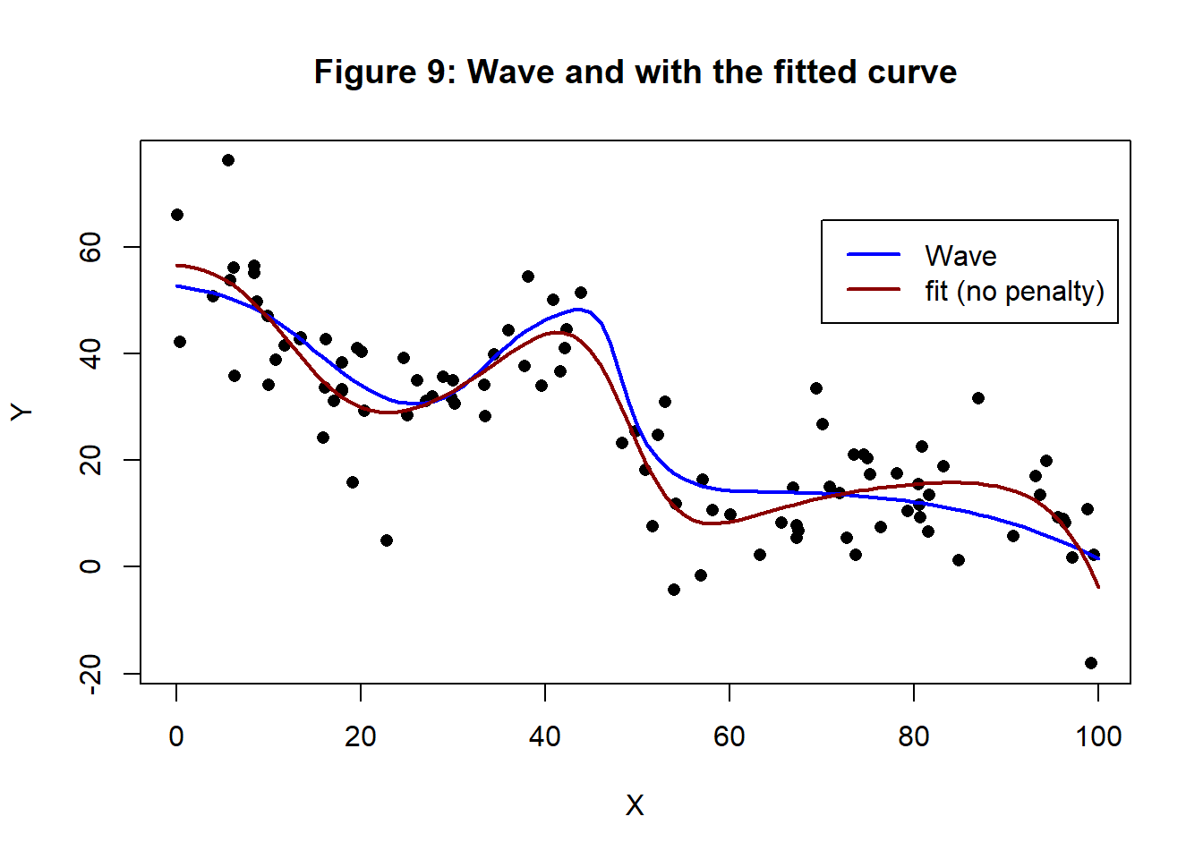
The fitted biases of the 8 hidden nodes and 1 output node are
## [1] 6.00 -13.92 2.42 -0.76 -0.80 3.85 8.67 7.37The weights are
##  [1]   2.60  24.07   4.61 -28.82  -9.35  -0.12  20.22   6.11  -4.72 -13.57
## [11]   5.53  13.43 -11.82  -2.05  -9.18  -2.59
The first 8 weights connect the input, X, to the hidden nodes and the next 8 weights connect the hidden nodes to the output, Y.
We might take the view that this model is too wavy and that it probably overfits. Of course, you must reach this conclusion based on external information, because in practice, you will not know the true shape of the wave. Anyway, you might decide to limit the sizes of the weights and biases. The model produced without penalisation has parameters between about -25 and 25, an approximate standard deviation of 10. Let’s assume that you decide that -10, 10 is a more reasonable range, a standard deviation of about 5. So lambda for the L2 penalty should be roughly \(2.5/5^2=0.1\).
Figure 10 shows the pattern of reduction of the penalised loss (MSE+Penalty) and the MSE component of the loss. The MSE of the unpenalised analysis is shown for comparison.
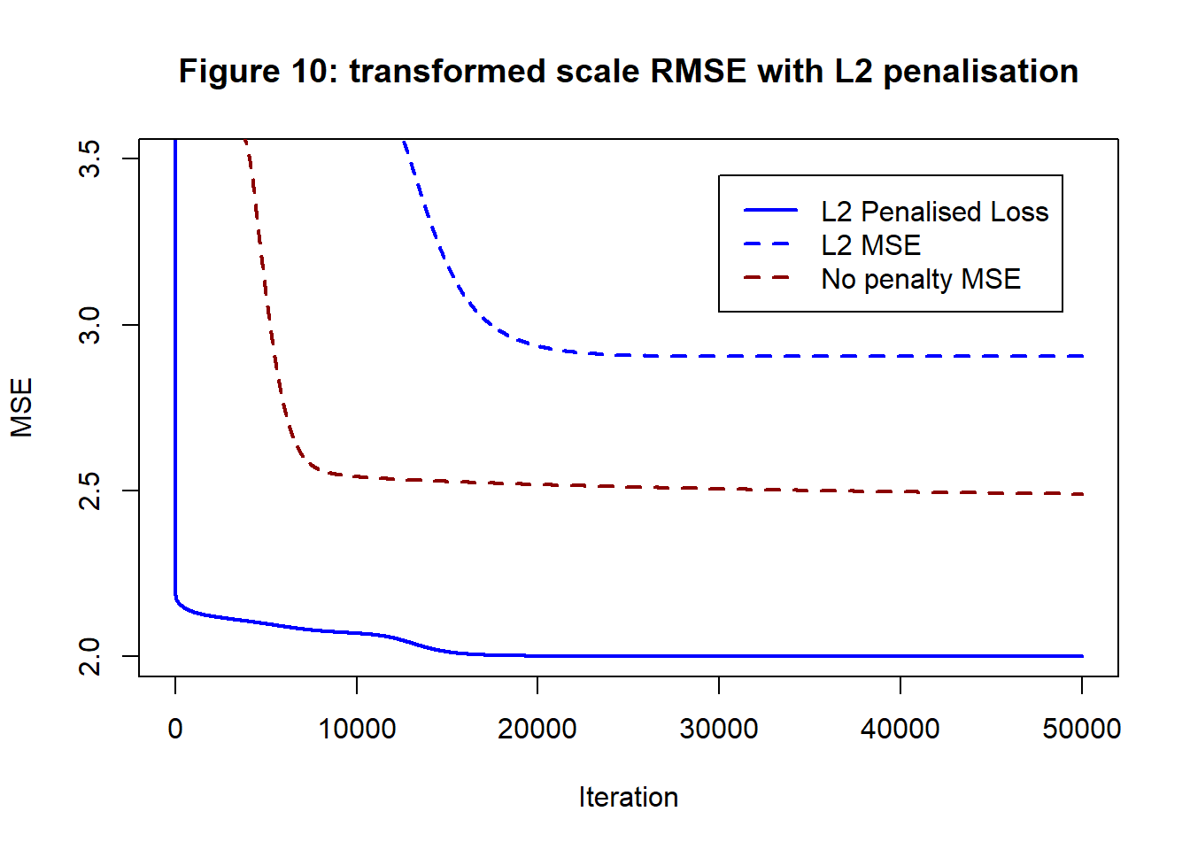
The MSE component of the loss now drops to 2.9, while the total penalised loss drops to 4. The training MSE is not as low as before meaning that the curve will less closely follow the training data.
The new biases are
## [1] 0.00 -3.71 0.31 -0.50 -1.00 0.00 5.92 0.01and the new weights are
##  [1]   0.00   6.91   5.87 -19.62  -7.24   0.00  12.87   0.03   0.00  -5.85
## [11]   6.04  11.23  -7.38   0.00 -10.21   0.03
These values are broadly in line with what I intended. In figure 11, the new fitted curve is shown in purple, with the unpenalised curve is in brown. The penalised algorithm does produce a slightly less wavy curve.
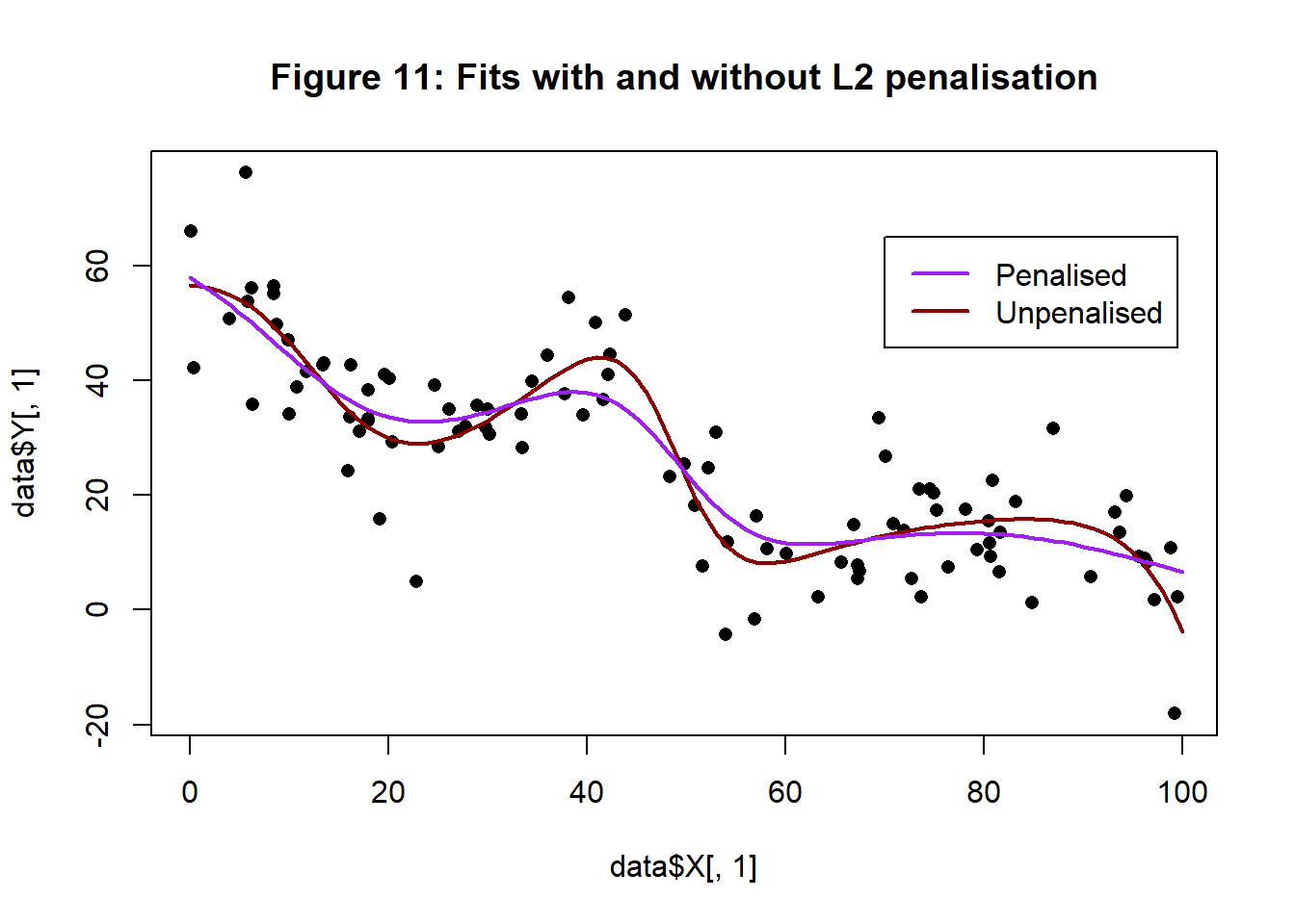
The test MSE of the predictions from the unpenalised model is 79.204 while for the penalised model the test MSE is 82.182, which means that penalisation has made the test performance slightly worse.
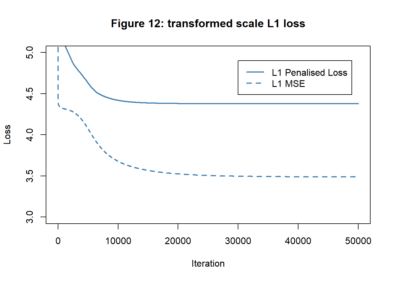
For comparison, I will also try L1 penalisation. In an attempt to make the effect dramatic, I opted for a large value of lambda and ran the algorithm with \(\lambda=1.45\).
The new biases are
## [1] 0.00 0.00 0.00 -0.29 0.00 0.00 7.82 0.00 1.62and the new weights are
##  [1]   0.00   0.00   0.00 -25.98   0.00   0.00  15.93   0.00   0.00   0.00
## [11]   0.00   4.41   0.00   0.00  -5.35   0.00
The Laplace has had the desired effect of making most of the weights and biases zero. In fact only, nodes 4 and 7 are used at all to create the fitted curve and we might just as well have used a neural network with a (1, 2, 1) architecture. Figure 13 shows the L1 fit with the L2 fit and unpenalised fit for comparison.
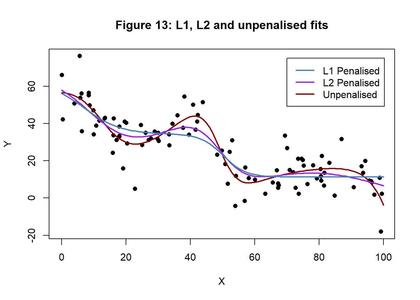
The test MSE for the L1 penalised model is 96.507. In this example, it looks as though L1 penalisation has over-done the damping of the curve, but I did try for a dramatic effect.
A massively over-parameterised model
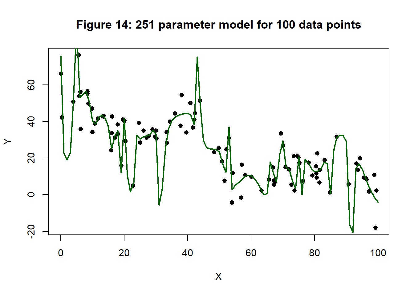
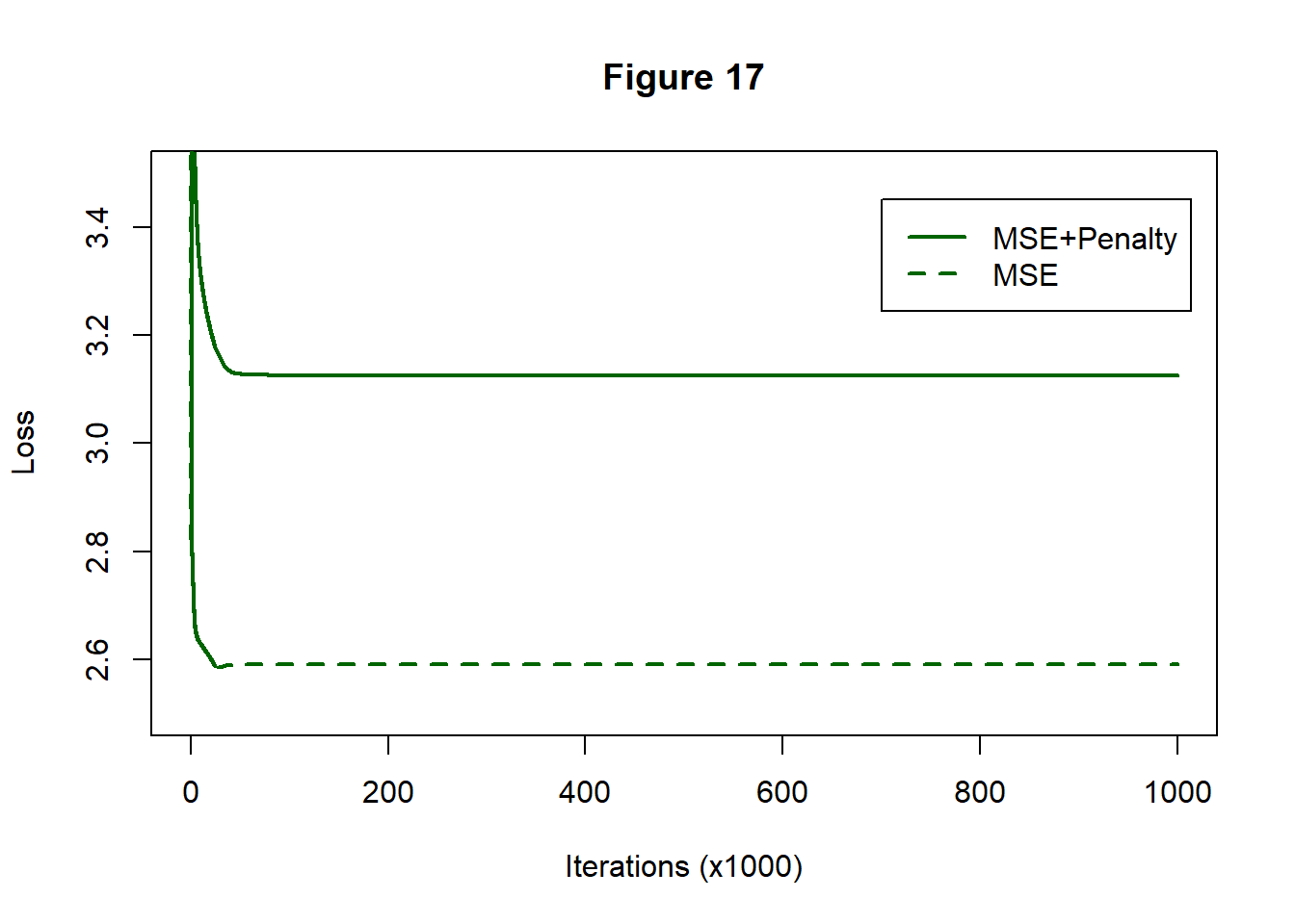
In this section, I fit a (1, 10, 10, 10, 1) neural network to the same set of training data. This model has 251 parameters, more than there are points in the training data (100). I fitted by gradient descent with one million iterations and a step length that started at 0.1 and dropped by 10% every 50,000 iterations. Figure 14 shows a plot of the resulting fit.
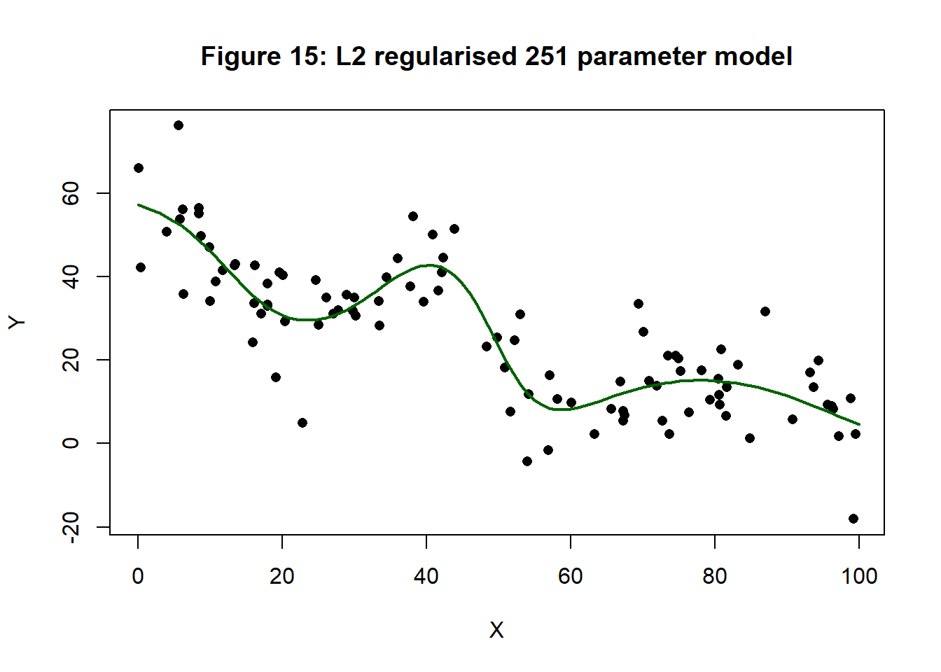
At last we have a real candidate for regularisation. I used L2 regularisation with lambda = 0.1. As we saw previously, this is roughly equivalent to a variance of 25 for the parameters, that is to say, a standard deviation of 5, or most weights in the range (-10, 10). The algorithm was again run for one million iterations. Figure 15 shows the resulting fit.
The effect is remarkable. Figure 16 shows a histogram of the 220 weights for the models with (dark blue) and without (light blue) L2 penalisation.
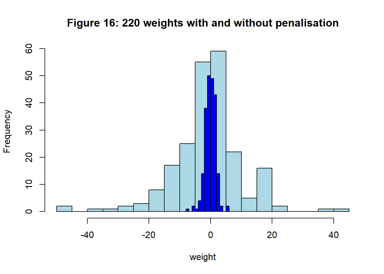
Figure 16 shows the reduction in the loss; there is not much changes after about 100,000 iterations. The MSE component flattens out at about 2.6 quite close to the MSE of the unpenalised NN(1, 8, 1). Interestingly, the test MSE is 77.202, which is better than any of the other models tried so far.
Conclusions
Here are the points that I take from this investigation
- the machine learning literature needs to be clearer about its terminology
- you might not like my definitions but at least I have tried
- regularisation is not just about overfitting
- we should embrace the subjectivity in our data analyses and be proud of using external information
- when we use external information or extra assumptions, we need to be explicit
- regularisation is essential when a model is ridiculously over-parameterised
- it is not good practice to use ridiculously over-parameterised models
Appendix: Code Changes
The C code used in this post can be found on my GitHub pages as cnnUpdate03.cpp.
I added options to cfit_nn() and cfit_valid_nn() to allow
- L1 and L2 regularisation
- separate lambdas for weights and biases
- other penalty functions by modifying the
cpenalty()&cdpenalty()functions
I have removed the etaAuto option that reduced the step length when the loss increases. Experience showed that short periods of rising loss are often needed before the algorithm makes progress. etaAuto stopped the algorithm too soon. I need to find a way to make the automatic adjustment more intelligent.