Neural Networks for Classification II: Assignment Rules
Introduction
This the ninth in a series of posts in which I am developing a workflow for using neural networks in data analysis by experimenting with small simulated datasets. In my last post, I adapted my regression-based workflow so that it could be applied to classification problems and I was at pains to stress the similarity between regression and classification; both predict an average, in one case the average of the response variable and in the other, the probability of class membership, which is the average response when items in the class are scored 1 and items out of the class are scored 0.
Although the methods for modelling classification and regression are very similar, there is one important difference; in classification problems, the class probabilities estimated by the model usually need to be turned into class assignments using an assignment rule. This extra step might be buried within the model itself, or it might be done later by the analyst.
For some problems, the extra step of class assignment is trivial. Imagine that there are two classes and that for a given set of features, your model allocates a probability of 0.8 to the first class and 0.2 to the second class. Common-sense says that the item should be assigned to the first class. Indeed, an assignment rule that puts each item into the class with the larger, or largest, probability will maximise the overall accuracy. This natural assignment rule is optimal for many problems, but not for all. I will discus some cases when this natural choice is not appropriate.
One of the scenarios that I’ll discuss is that of imbalanced training data, that is, data in which some classes are much less common than others. A popular machine learning technique for handling imbalanced training data is over-sampling, which works by implicitly changing the assignment rule. Whenever a method makes implicit changes, I, for one, get nervous; it is always difficult to make rational choices when the consequences of your decision is a side-effect, or when they are hidden away in the detail. I suspect that over-sampling is often used without really understanding its impact.
The Larger Probability Assignment Rule
Typically, a neural network will take features X as its input and output estimates of the class probabilities P(Class k | X), k=1,..,K. Often these probabilities are only part of the solution and we also need to assign new items to their most appropriate class and to measure the performance of that assignment.
Let’s look at a general two-class problem and the population from which the training data were drawn. The larger probability assignment rule says that for any set of features X, we should assign to class 1 whenever, \[ P(Class \ 1 \ | \ X) > P(Class \ 0 \ | \ X) \] Bayes theorem tells us that this is equivalent to, \[ P(X \ | \ Class \ 1) \ P(Class \ 1) > P(X \ | \ Class \ 0) \ P(Class \ 0) \] The first term on each side of the inequality describes the distribution of the features in that class and the second term describes the proportion of the population that are from that class.
The boundary between the assigned classes lies through the points, X, where \[ P(Class \ 1 \ | \ X) = P(Class \ 0 \ | \ X) \] or equivalently, where \[ P(X \ | \ Class \ 1) \ P(Class \ 1) = P(X \ | \ Class \ 0) \ P(Class \ 0) \] This boundary divides the space of features, X, into two regions, which I’ll refer to as \(R_1\) for the region within which items are assigned to Class 1 and \(R_0\) for the remainder of the space, where assignment is to class 0.
This boundary is optimal in the sense of minimising the number of assignment errors, but its use will still make errors. The performance of the rule is described by two values, the sensitivity and specificity. The sensitivity is the probability of correctly assigning items that come from class 1 \[ Sensitivity = \int_{R_1} P(X \ | \ Class \ 1) dX \] The specificity is the probability of correctly assigning items that come from class 0 \[ Specificity = \int_{R_0} P(X \ | \ Class \ 0) dX \] Obviously, there is a symmetry between sensitivity and specificity depending on which class you label as 0 and which you label as 1. Usually, people use the label 1 for the class that they are primarily interested in, but it is arbitrary.
Given the sensitivity and specificity, we can derive other performance measures. For example, the overall accuracy is the probability of making the correct assignment \[ Accuracy = P(Class \ 1) Sensitivity + P(Class 0) Specificity \]
Other Assignment Rules
The larger probability assignment rule can be generalised by multiplying the class probabilities by weights, \(W_k\), before they are compared. The weighted assignment rule would assign to class 1 whenever, \[ W_1 P(Class \ 1 \ | \ X) > W_0 P(Class \ 0 \ | \ X) \] Obviously, \(W_1\) = \(W_0\) corresponds to the larger probability assignment rule and \(W_1\) > \(W_0\) moves the boundary so that \(R_1\) is larger and more items are assigned to class 1, while \(W_1\) < \(W_0\) favours assignment to class 0.
In all but pathological cases, increasing the size of \(R_1\) will cause the sensitivity to increase and the specificity to decrease. Such a change would be appropriate for scenarios in which it is more important to correctly identify items from class 1, as opposed to items from class 0.
A second scenario in which it makes sense to move the boundary is when you want to apply the model to target data from a new population in which the distributions of the features, P(X | Class 1) and P(X | Class 0), are the same as in the training set, but the class frequencies, P(Class 1) and P(Class 0) are different.
Mechanisms for moving the assignment boundary
We have seen how the position of the assignment boundary can be moved by introducing Weights, \(W_k\), into the comparison of the estimated class probabilities, but there are two other ways of achieving the same end result; these involve, either modifying the loss function, or modifying the training data.
Let’s start by changing the loss function. The standard K-class cross-entropy loss is \[ Loss(y, \hat{y}) = - \frac{1}{n} \sum_{i=1}^n \sum_{k=1}^K y_{ik} log(\hat{y}_{ik}) \] where \(\hat{y}_{ik}\) is the estimated value of \(P(Class \ k \ | \ X_i)\).
This loss function can be generalised by introducing class weights (or class costs), \(W_k\), so that the loss becomes \[ Loss(y, \hat{y}) = - \frac{1}{n} \sum_{i=1}^n \sum_{k=1}^K W_k y_{ik} log(\hat{y}_{ik}) \] A large value of the weight for a given class will increase the contribution to the loss of items from that class and consequently the algorithm that minimises the loss will try to classify that class correctly at the expense of items from other classes. The modified loss function will change the predicted class probabilities and class assignment can be based on the larger of these new probabilities.
The other alternative is to change the proportion of each class in the training data. Suppose that we were to sample a fraction, \(W_k\), of the data on class k, then the larger probability boundary would move to \[ P(X \ | \ Class \ 1) \left\{ W_1 P(Class \ 1) \right\} = P(X \ | \ Class \ 0) \left\{ W_0 P(Class \ 0) \right\} \] If the sampling faction, \(W_k\), is less that one, this is referred to as under-sampling, since not all of that class’s training data are used, while if the fraction is greater than 1, it is referred to as over-sampling, as some of the training data will be used more than once.
Selecting an assignment rule
Choosing a good assignment rule is critical to the success of any classification analysis and to understand why, we will need a range of measures of the performance of the assignment, these include the accuracy, sensitivity, specificity and the ROC curve. I’ll introduce these performance measures using simulated data and then I’ll show how the performance measures are affected when the assignment rule is changed.
I’ll base the simulations on two scenarios that require a change in the assignment rule.
Scenario 1
In the first simulation, I imagine that I have training data on 100,000 UK births and that I want to predict a condition in the babies that has a prevalence of about 15%. The chance of the baby being affected by the condition depends on the mother’s age and the quality of the mother’s diet. Having developed the model and measured its performance, I’ll imagine applying the UK trained model to the screening of babies in a very poor country with a more deprived diet. I’ll call this second country, South Sudan as I think that this is currently the world’s poorest country.
In this simulation, I will model the data using logistic regression rather than a neural network. Logistic regression is quicker to fit and the coefficients are more easily understood. Everything that I describe would apply equally to data modelled by a neural network, although a neural network would typically have smaller bias and larger variance.
Simulating the UK training data
First, I create a set of training data of 100,000 UK births by simulating maternal age and a measure of poor maternal diet. Those two features determine the probabilities that a baby has the condition (y=1), or does not have it (y=0). The simulated data are stored in a data frame called df_uk.
# Simulated UK training data
set.seed(3981)
df_uk   <- data.frame(
                diet = rgamma(100000, 0.5, 10),
                age  = rgamma(100000, 30, 1.1))
logit   <- -33 + 6 * df_uk$diet + df_uk$age
prob    <- 1 / (1 + exp(-logit))
df_uk$y <- rbinom(100000, 1, prob)
Figure 1 shows the distributions of the measure of poor diet and of maternal age. The important point is that in the UK, few mothers have a poor diet according to this measure. Yes, I know that UK diet is terrible, but not in the way being measured here.
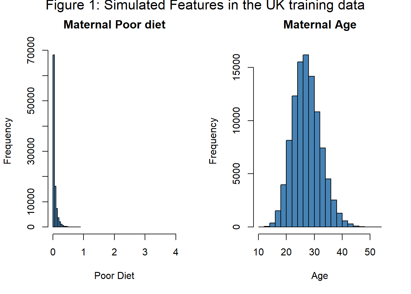
Table 1 summarises the frequency of the condition in the simulated training data and confirms that about 15% of babies have the condition.
| Table 1: Prevalence of the condition in the UK | ||
| True Class | Number | Percentage |
|---|---|---|
| 0 | 84654 | 84.7 |
| 1 | 15346 | 15.3 |
Now, I fit a logistic regression model to the simulated data. As you would expect with such a large training set, the estimated coefficients are very similar to those used in the simulation. The coefficient of diet is less well estimated than the age coefficient, because this measure of diet does not vary much in the UK population.
| Table 2: UK logistic regression coefficients | |||
| term | estimate | std.error | p.value |
|---|---|---|---|
| (Intercept) | −32.9527 | 0.2922 | 0.0000 |
| age | 0.9994 | 0.0090 | 0.0000 |
| diet | 5.9153 | 0.2038 | 0.0000 |
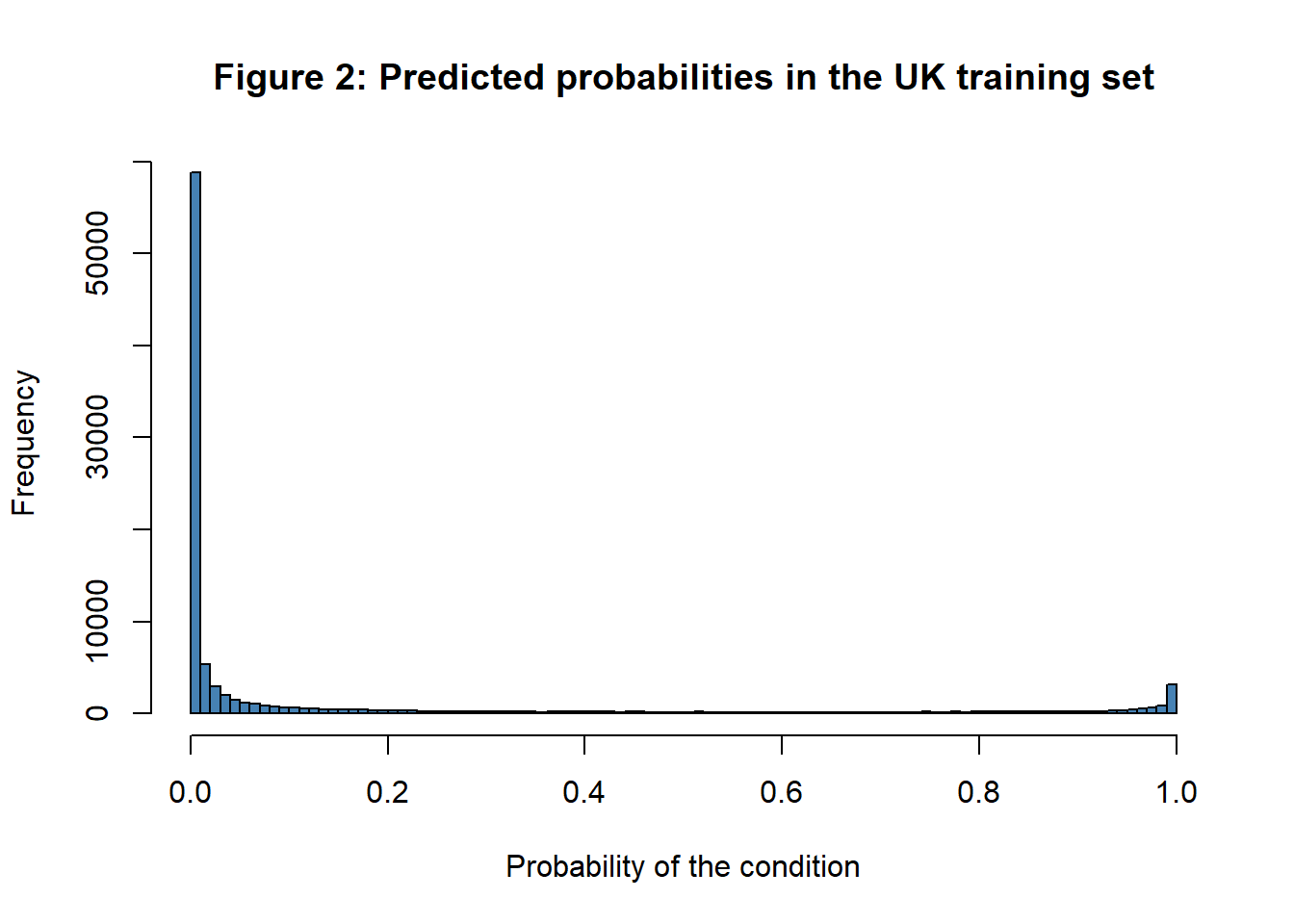
If we look at the probabilities predicted by the model, they also follow the pattern that we would expect, with most probabilities close to 0 or 1. Overall, the model does a good job of predicting the condition. The average of the probabilities predicted by the model is 0.153, which corresponds to the prevalence of the condition in the UK.
The obvious assignment rule to use is the “larger probability”. The confusion matrix for this rule shown in table 3, it contains counts of babies by their true class and their assigned class.
| Table 3: Logistic regression confusion matrix based on larger probability assignment |
||
| True Class | Predicted Class | |
|---|---|---|
| 0 | 1 | |
| 0 | 82578 | 2076 |
| 1 | 3431 | 11915 |
The confusion matrix shows that (82,578+11,915)/100,000, or 94.5% of babies are correctly classified by this rule, this the overall accuracy . Amongst babies with the condition, 11,915/(11,915+3,431), or 77.6% are correctly identified, this is the sensitivity of the assignment rule, and amongst babies who do not have the condition 82,578/(82,578+2,076), or 97.5% are correctly identified, this is the specificity.
Introducing class weights would create a different assignment rule. For instance, if we chose \(W_1\)=1 and \(W_0\)=0.25, the rule would assign to class 1 whenever \[ P(Class \ 1 \ | \ X) > 0.25 P(Class \ 0 \ | \ X) \] This new rule would reduce the number of babies classified as being healthy (class 0), which would reduce the specificity, but the sensitivity would increase.
Using this particular weighted assignment rule the confusion matrix becomes,
| Table 4: Logistic regression confusion matrix for an assigment rule with weights 0.25 and 1 |
||
| True Class | Predicted Class | |
|---|---|---|
| 0 | 1 | |
| 0 | 78226 | 6428 |
| 1 | 1364 | 13982 |
For this rule, the accuracy is 92.2%, the sensitivity is 91.1% and the specificity is 92.4%. Both the accuracy and the specificity are slightly worse than under the unweighted rule, but the sensitivity has improved a lot. The rule is better at identifying babies with the condition, but worse at identifying healthy babies. Only you can decide whether that is what you want.
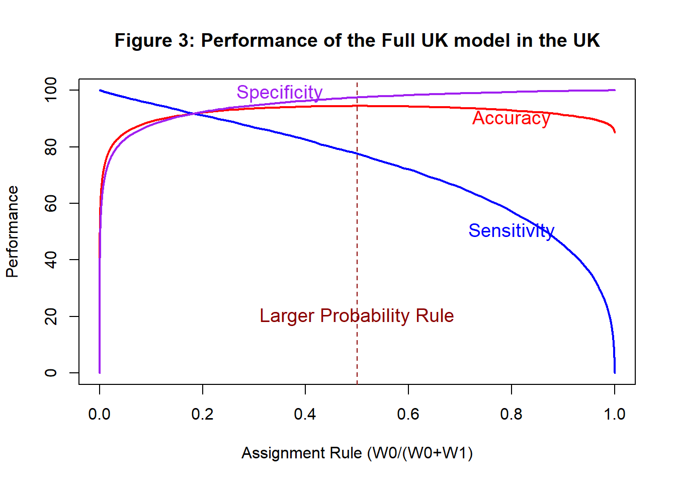
Figure 3 shows the way that the performance measures change as the assignment rule is changed. The x-axis shows the value of \(W_0/(W_0+W_1)\), so the larger probability rule corresponds to a value of 0.5; this maximises the overall accuracy. A rule based on \(W_0\)=0 (every baby is classified as having the condition) would maximise sensitivity and a rule based on \(W_1\)=0 (every baby is classified as healthy) would maximise specificity.
The balance between sensitivity and specificity is usually shown by plotting the ROC (Receiver Operating Characteristic) curve. For historical reasons, an ROC curve plots sensitivity against 100-specificity, but unhelpfully, the sensitivity is often referred to as the true positive rate and 100-specificity is called the false positive rate.
Every possible assignment rule corresponds to a particular point (combination of sensitivity and specificity) on the ROC curve. Figure 4 shows the UK model’s ROC curve and highlights the point corresponding to the larger probability rule.
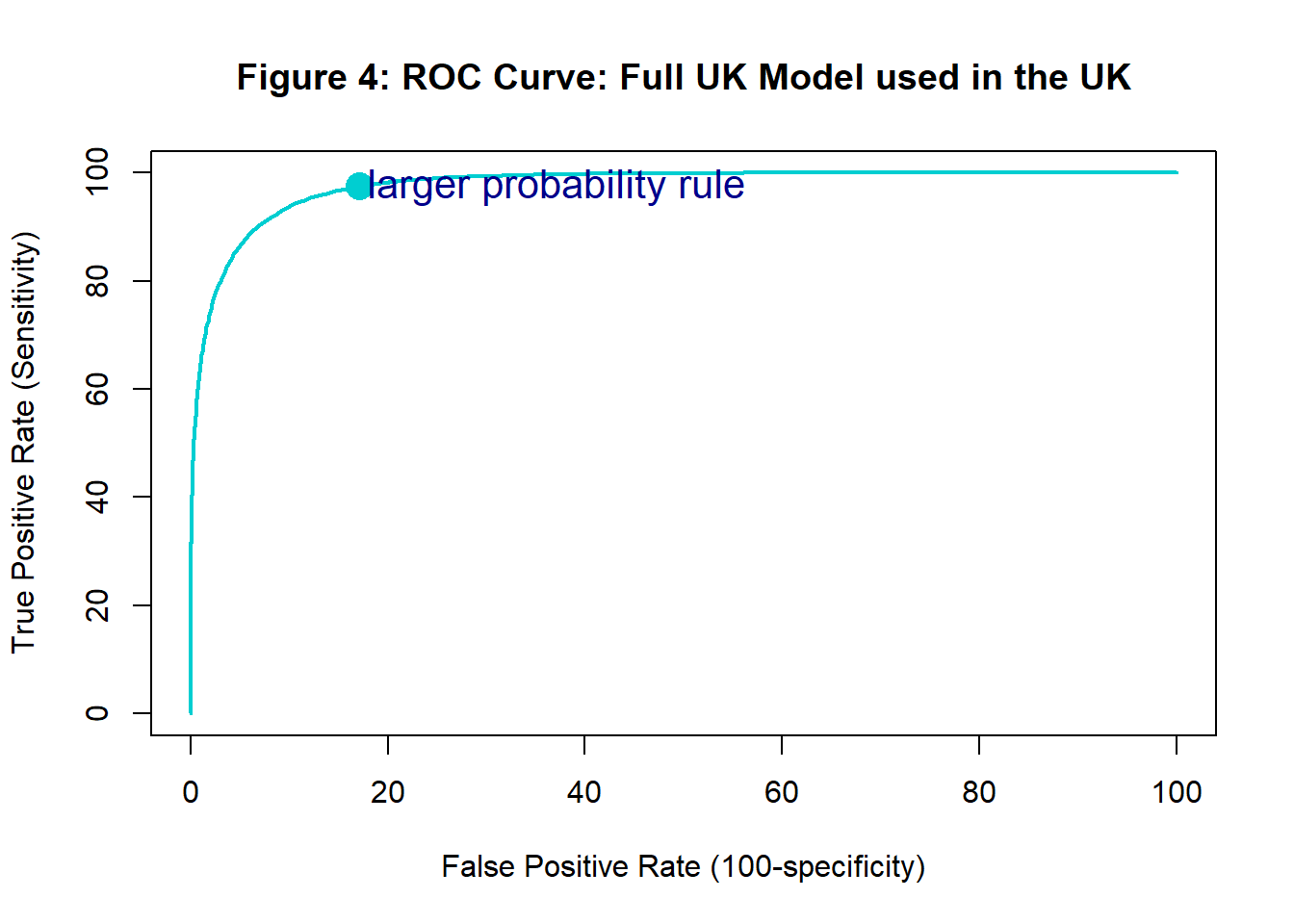
The important point to remember is that the predicted probabilities determine the ROC curve and the assignment rule selects a point on that ROC curve. Each point on the ROC curve corresponds to a different assignment rule applied to the same set of predicted probabilities.
Sometimes the area under the ROC curve, called the AUC, is used as a measure of performance. Since the shape of the ROC curve only depends on the predicted probabilities and not the assignment rule, this is a measure of the quality of the predicted probabilities and not of the quality of the assignment. The AUC even has a probability interpretation, take a random item from class 1 and a random item from class 0, the probability that the item from class 1 has the higher predicted probability of being in class 1 is equal to the AUC. This interpretation is mathematically appealing, but not of much practical use. More useful is the idea that a large AUC is a good thing, because it implies that there must be an assignment rule with both a high sensitivity and a high specificity.
The simulated measure of poor diet does not change much in the UK, so quite possibly researchers would not bother to measure it. In that case, the condition would have to be predicted from maternal age alone. Table 5 shows the coefficients of this logistic regression.
| Table 5: Age only Logistic regression | |||
| term | estimate | std.error | p.value |
|---|---|---|---|
| (Intercept) | −31.6474 | 0.2765 | 0.0000 |
| age | 0.9685 | 0.0086 | 0.0000 |
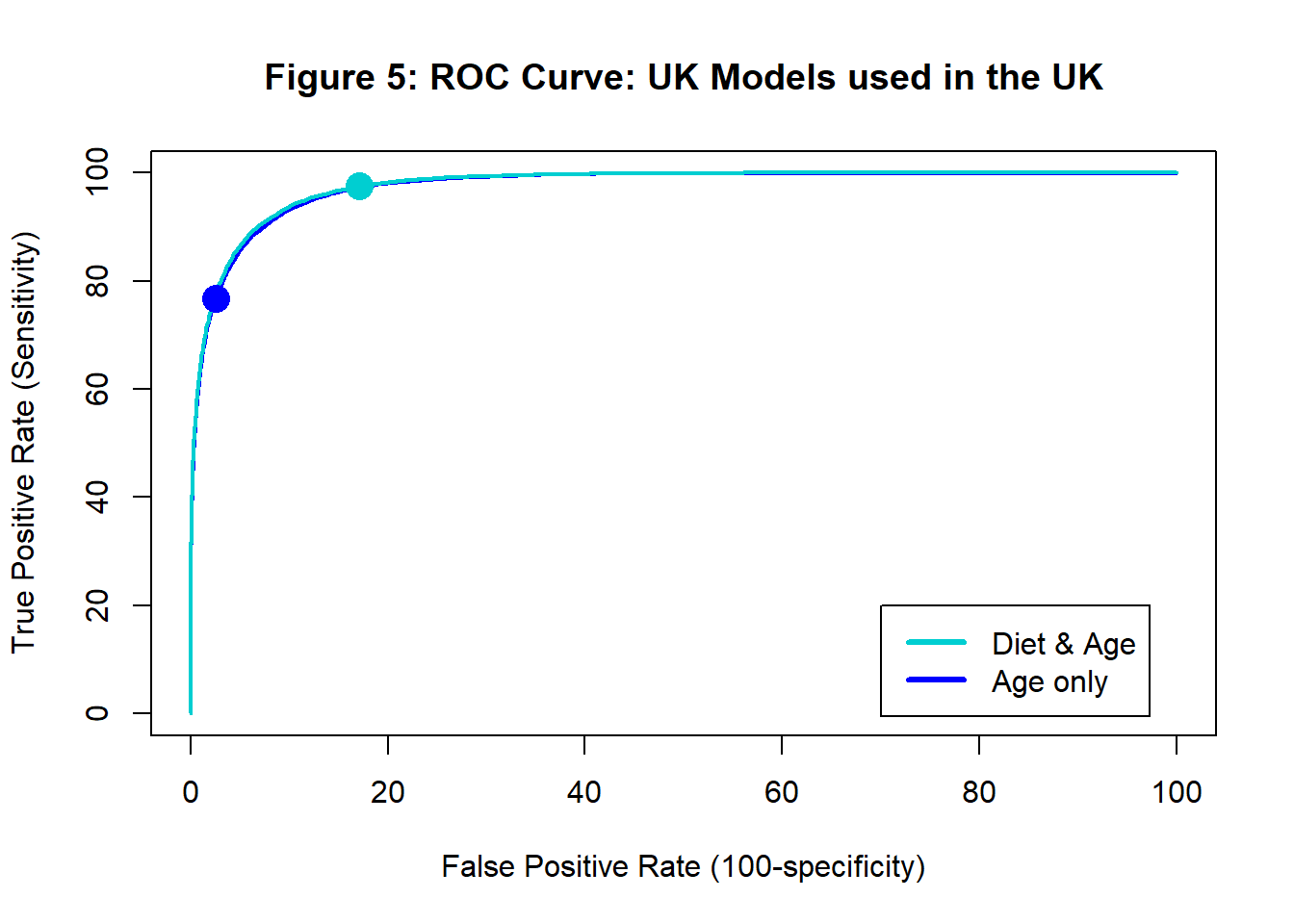
Figure 5 shows the ROC curve for the age only model with the ROC curve of the original (age and diet) model shown in a lighter blue. The points corresponding to the the “larger probability rule” are highlighted. The difference between the performances of the models as measured by the AUC is tiny, because the measure of poor diet does not vary much in the UK.
South Sudan
Now let’s imagine taking the UK models, with and without diet, and using them to predict the same condition in South Sudan. The code below simulates 100,000 imaginary South Sudanese births.
set.seed(2884)
df_ss  <- data.frame(
   diet      <- rgamma(100000, 5, 5),
   age       <- rgamma(100000, 34, 1.3)
)
logit     <- -33 + 6 * df_ss$diet + df_ss$age
prob      <- 1 / (1 + exp(-logit))
df_ss$y   <- rbinom(100000, 1, prob)
Figure 6 shows that a poor diet is much more common in this simulated sample than it was in the simulated UK data.
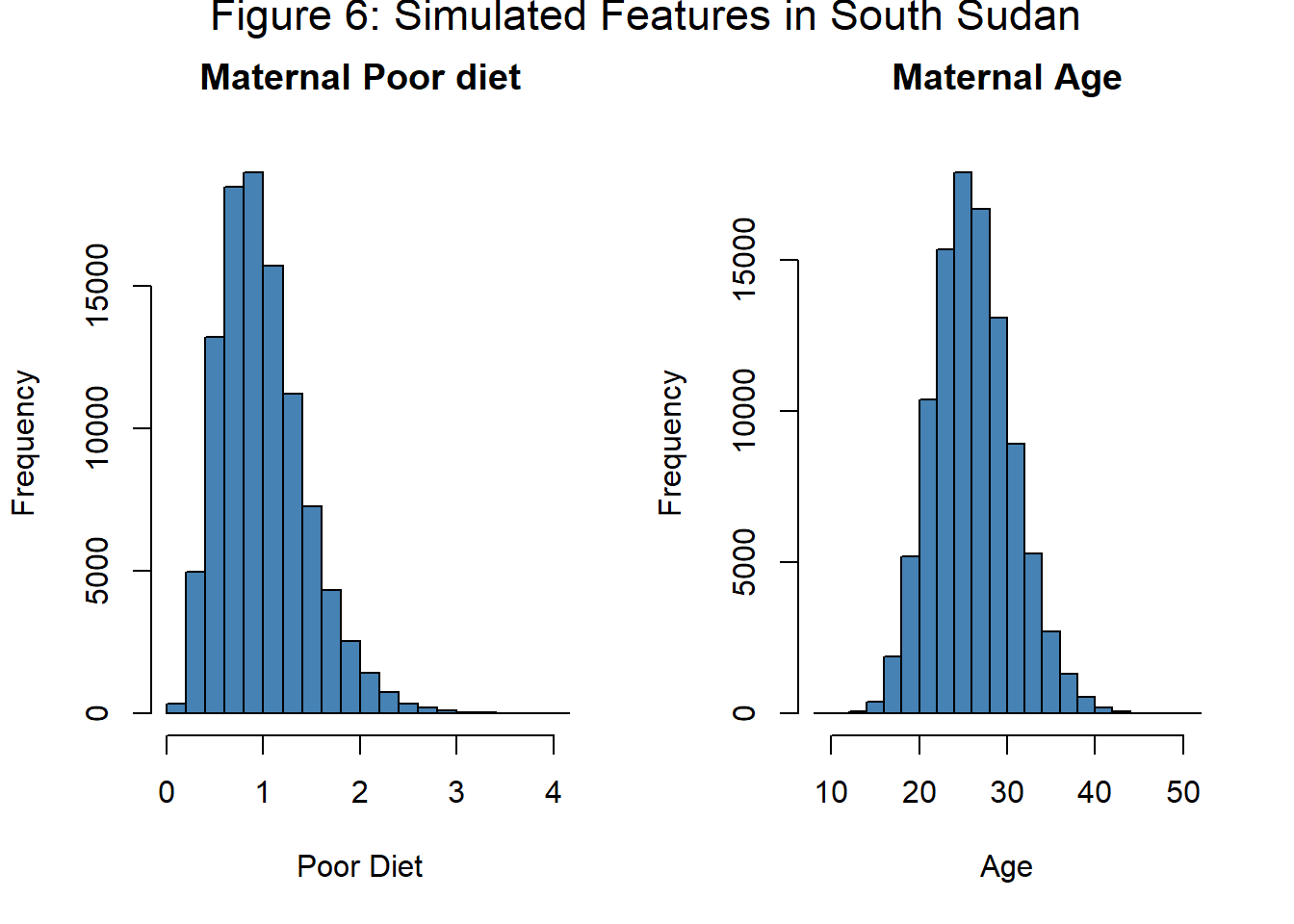
In the South Sudanese simulation, I assume that the impact of age and diet on the condition (the model coefficients) are the same as in the UK, it is just that the diet is worse in South Sudan, so the prevalence of the condition is higher; table 6 shows that this prevalence is close to 42%.
| Table 6: Prevalence of the condition in South Sudan | ||
| True Class | Number | Percentage |
|---|---|---|
| 0 | 58232 | 58.2 |
| 1 | 41768 | 41.8 |
The question that we need to answer is, if we were to use the UK trained models to screen for the condition in South Sudan, would it be sensible to use the same assignment rule as in the UK?.
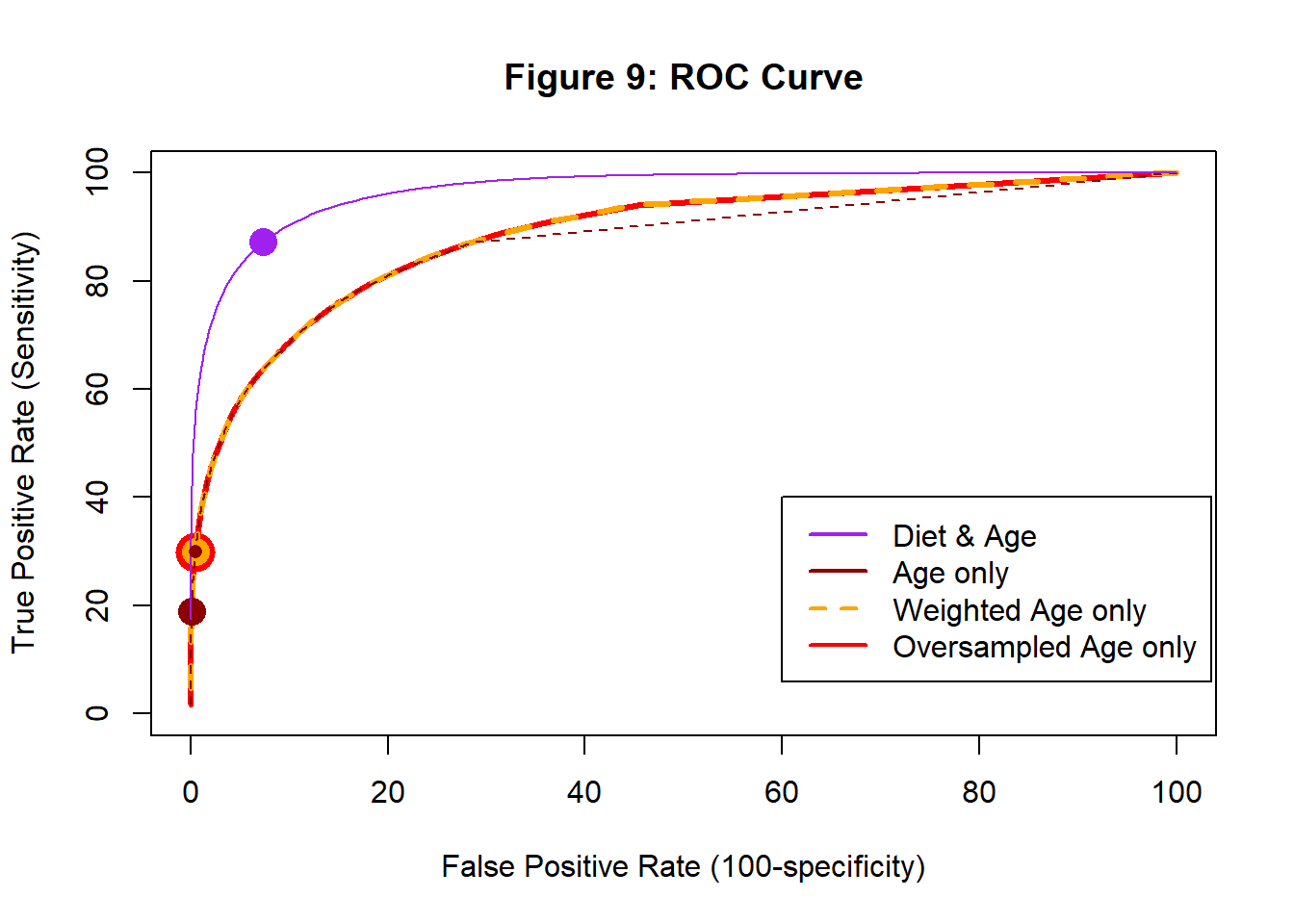
The plot below shows the performance of the two models trained on UK data (age only and age+diet) when used on the simulated South Sudanese births. As usual, the highlighted points correspond to the larger probability assignment rule.
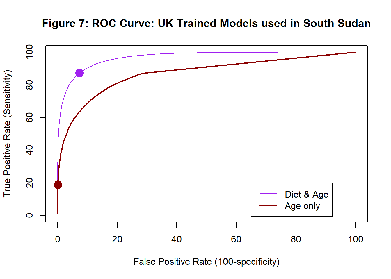
The model that includes diet does very well in South Sudan and the “larger probability” assignment rule provides a good compromise between sensitivity and specificity.
In the UK, the models with and without diet performed more or less equally well, but in South Sudan the model without diet performs much worse and the “larger probability” rule would identify under 20% of the babies with the condition. The age only model is calibrated for use in the UK not South Sudan, but perhaps a different assignment rule would help correct for the miscalibration. Looking at the ROC curve, it seems that it would be possible to find an assignment rule for use with the age only model that has specificity and sensitivity that are both close to 80%.
Weighted Class Probabilities
How do we make the age only model suitable for use in South Sudan? We know that the prevalence of the condition in the UK is about 15%, Imagine that we found a study that reported a 40% prevalence in South Sudan. The probability of being in class 1 needs to be adjusted from 15 to 40 and the chance of being in class 0 needs to change from 85 to 60. \[ (40 / 15) P(Class \ 1 \ | \ X) > (60 / 85) P(Class \ 0 \ | \ X) \]
Using this weighted rule the sensitivity becomes 30% and the specificity becomes 99.5%. This is optimal in terms of overall accuracy, but I suspect that many people would opt for an even stronger weighting that would increase the sensitivity still further at the expense of the specificity.
Sample weights
We could create sampling weights for the UK data and refit the age only model.
weight    <- (df_uk$y == 0 ) * 60 / 85 + (df_uk$y == 1) * 40 / 15
mod_ukw   <- glm(y ~ age, family=binomial(), data=df_uk, weights=weight)
The sampling weights make the model assume that the UK sample had more babies with the condition and as a result, the weighted logistic regression creates a new model with predicted probabilities calibrated for use in South Sudan.
| Table 7: Weighted Logistic regression on UK data | |||
| term | estimate | std.error | p.value |
|---|---|---|---|
| (Intercept) | −30.2126 | 0.2212 | 0.0000 |
| age | 0.9651 | 0.0070 | 0.0000 |
When we look at the ROC curve of the weighted model it is identical to the unweighted ROC curve.
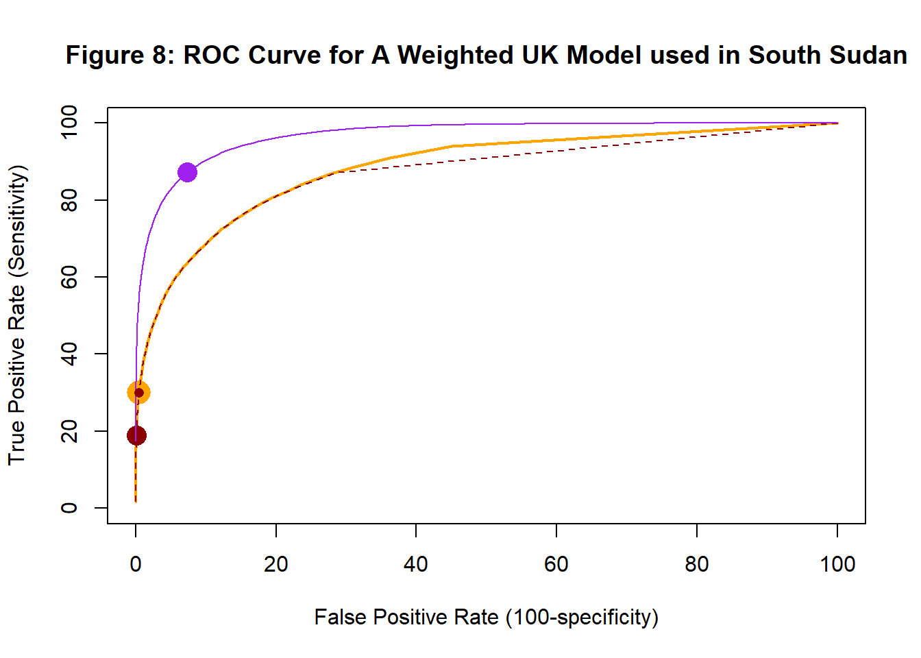
The weighted and unweighted models are different. They have different model parameters and they make different probability predictions, yet the performance profiles are the same, i.e they have the same ROC curve. They produce differently calibrated predicted probabilities and the point corresponding to the larger probability rule moves along the common ROC curve when the model is weighted, from the large brown dot to the large orange dot.
The small brown dot inside the larger orange dot represents the combination of sensitivity and specificity that I got by using a weighted class probability assignment rule. Instead of re-analysing the UK data with weights in the loss function, I could just as well use the original UK model predictions and weight the assignment rule.
Let me finish with an apology, in figure 8 the the curves appear to diverge when the false positive rate exceeds about 30%; this is an artefact of the simulation. To get better agreement, I would have had to simulate millions of babies and I could not be bothered. Theoretically, the ROC curves are the same.
Over-sampling
An alternative to weighting would be to sample babies from the UK training data so that the proportion with the condition resembles that found in South Sudan. This would require under-sampling the babies without the condition and over-sampling the babies with the condition. In the next analysis, I randomly sample 40,000 UK babies with the condition and 60,000 without and then refit the model. This is almost identical to using a weighted loss, the only difference lies in the randomness of the sampling. Weighting always gives the same model, over and under-sampling create very slightly different models each time a different sample is drawn.
set.seed(9482)
smp    <- c(sample(which(df_uk$y == 0), 60000, replace=FALSE),
            sample(which(df_uk$y == 1), 40000, replace=TRUE) )
df_uks <- df_uk[smp, ]
The regression coefficients are the same as those in the weighted analysis, hence the predicted probabilities will be the same.
| Table 8: Logistic regression for weighted UK samples | |||
| term | estimate | std.error | p.value |
|---|---|---|---|
| (Intercept) | −30.0601 | 0.2210 | 0.0000 |
| age | 0.9597 | 0.0070 | 0.0000 |
The ROC curves of the weighted and under/over-sampled models are identical. This is difficult to show in a plot because one curve disappears under the other. I’ve made the over-sampled lines and points a little bigger in the hope that you will see that both have been drawn.
Recap: Points to take from this simulation
I have covered a lot of ground, so let me recap the main points.
- The scenario concerned the prediction of a condition for which poor diet is an important predictor, but poor diet is uncommon in the training sample
- In the UK, models with and without poor diet perform almost equally well
- In South Sudan, the UK trained model that includes diet predicts well, but the UK trained model without poor diet predicts much less well
- The performance of an assignment rule is measured by the combination of that rule’s sensitivity and specificity
- The ROC curve shows the sensitivity and specificity of a model under different assignment rules
- The predicted probabilities determine the overall shape of the ROC curve
- Changing the assignment rule moves you to a different point on the ROC curve
- The “larger (unweighted) probability” assignment rule maximises overall accuracy in the training data
- Weighted comparisons, weighted loss & over/under-sampling calibrate the model for use in a different population
- Weighted comparisons, weighted loss & over/under-sampling are ways of reaching the same end point
- Sampling weights & over/under-sampling do not change the ROC curve
R’s glm() function allows sampling weights. To apply a weighted analysis to a neural network, you would have to incorporate the weights into the loss function so as to produce a weighted cross-entropy. This may not be possible if you are reliant on someone else’s software package, hence the popularity of under and over-sampling.
Scenario 2: A less common condition
In the second simulation, the condition being predicted still depends on diet and maternal age, but this condition is rarer and slightly more serious. The prevalence in the UK is about 1.5% and the model is only intended for screening babies in the UK. The factor that makes the scenario different is that detecting the condition at screening enables early treatment at a cost of £500 per baby, but delay will eventually require more expensive treatment costing £5000 per baby. Early treatment of a baby that turns out not to have the condition, does no long-term harm, but does incur the £500 cost.
Simulating the UK training data
The simulation is very similar, except that the intercept term in the simulation is much smaller.
# UK training data for the second scenario
set.seed(3981)
df_uk   <- data.frame(
                diet = rgamma(100000, 0.5, 10),
                age  = rgamma(100000, 30, 1.1))
logit   <- -40 + 6 * df_uk$diet + df_uk$age
prob    <- 1 / (1 + exp(-logit))
df_uk$y <- rbinom(100000, 1, prob)
Table 9 shows the prevalence in the simulated training data.
| Table 9: Prevalence of the second condition in the UK | ||
| True Class | Number | Percentage |
|---|---|---|
| 0 | 98466 | 98.5 |
| 1 | 1534 | 1.5 |
Table 10 gives the coefficients of the logistic regression model that uses both diet and age.
| Table 10: Logistic regression coefficients | |||
| term | estimate | std.error | p.value |
|---|---|---|---|
| (Intercept) | −39.9500 | 0.8358 | 0.0000 |
| age | 1.0000 | 0.0215 | 0.0000 |
| diet | 5.3285 | 0.5025 | 0.0000 |
Figure 12 shows the sensitivities and specificities
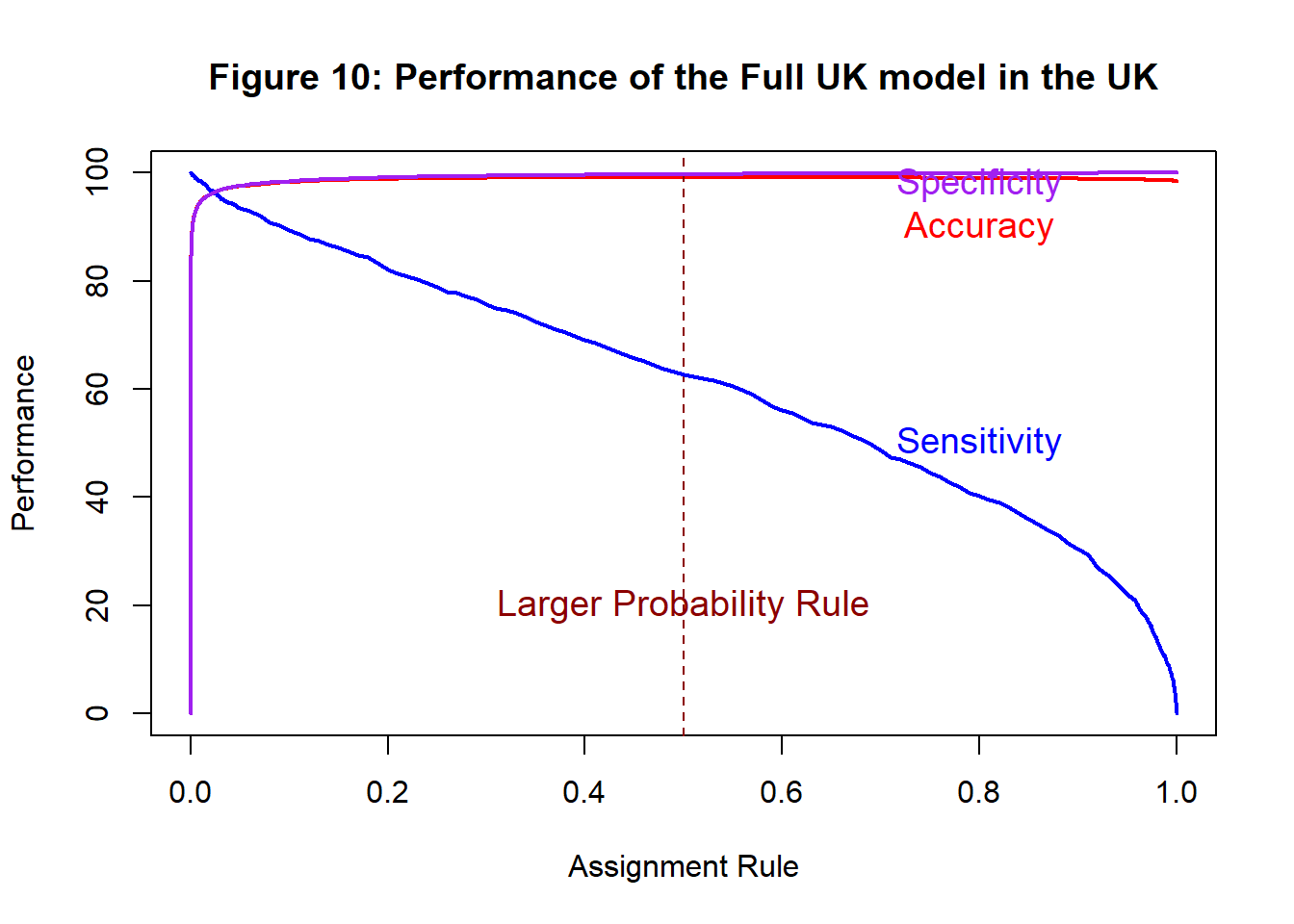
Figure 11 shows the ROC curve with the “larger” probability assignment rule highlighted.
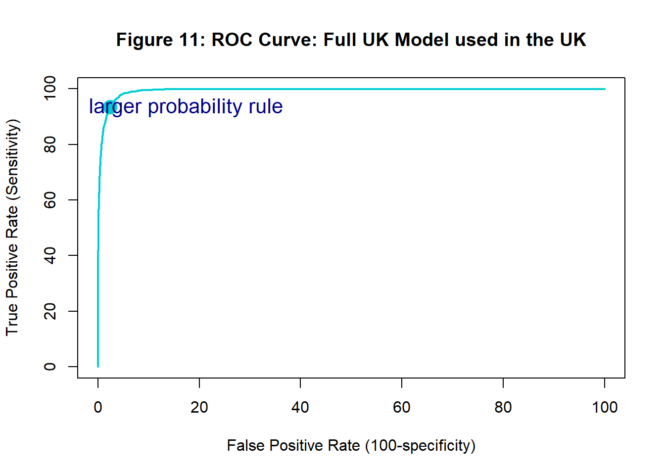
As always, the larger probability assignment rule maximises the overall accuracy.
| Table 11: Logistic regression confusion matrix | ||
| True Class | Predicted Class | |
|---|---|---|
| 0 | 1 | |
| 0 | 98224 | 242 |
| 1 | 572 | 962 |
The confusion matrix for the “larger probability” assignment rule shows that the model has an accuracy of 99.2 %. So it would make 812 or 0.8 % misclassification errors. No other assignment rule will reduce this number. However, the expected cost of implementing screening on 100,000 new births based on the larger probability rule would be (242+962)x500+572x5000=£3.462 million.
Suppose that we were to use an assignment rule based on weights \(W_1\)=1 and \(W_0\)=0.25. This is equivalent to the rule that says, whenever the chance of the condition (\(W_0/(W_0+W_1\)) is over 20%, we treat early.
| Table 11: Logistic regression confusion matrix | ||
| True Class | Predicted Class | |
|---|---|---|
| 0 | 1 | |
| 0 | 97623 | 843 |
| 1 | 274 | 1260 |
We now make more misclassifications, 1117 instead of 812, but more true cases of the condition are detected early and so the cost of this screening program is lower at (843+1260)x500+5274x5000=£2.742 million.
Using 1.5% as the prevalence, the average cost per baby of the program is 500x(0.015xsensitivity/100+0.985x(100-specificity)/100 )+5000x0.015*(100-sensitivity)/100. Figure 12 shows the cost in millions of screening 100,000 babies, using different assignment rules
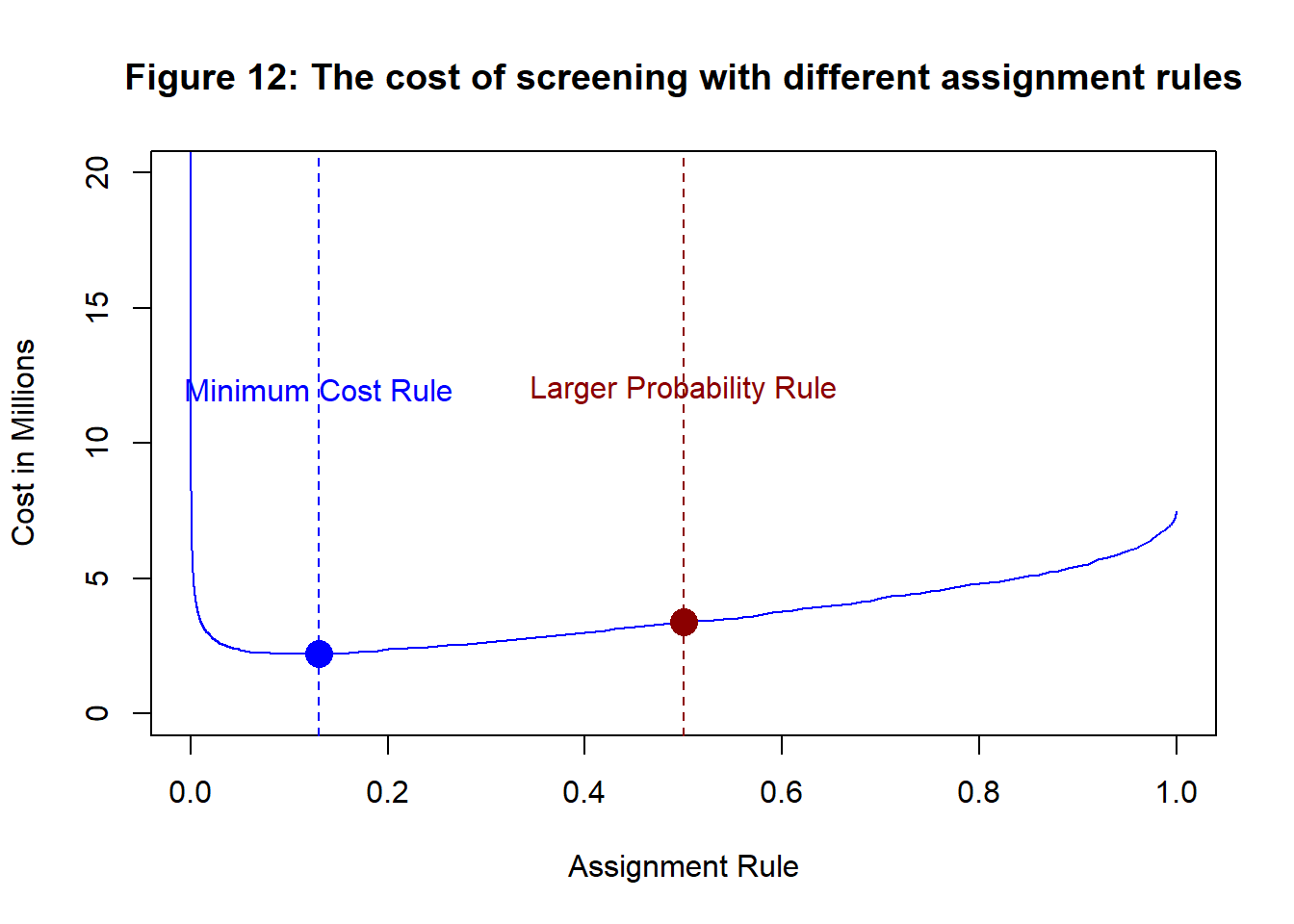
The minimum cost is £2.21 millions and it is achieved with an assignment rule that says, any baby with a predicted probability of having the condition that is greater than 0.13 should be treated early.
When we fit a model to the training data, we minimise the cross-entropy or in the case of logistic regression we maximise the binomial log-likelihood, which is equivalent. Minimising the cross-entropy will maximise the overall accuracy, but in this case we want to minimise cost and not the total number of misclassifications.
The most cost effective classification could be obtained from the predicted probabilities, as I have done here, or it could be found by modifying the loss function or by over/under- sampling.
Sample Imbalance
In my first post on classification, I analysed a kaggle dataset on cirrhosis in which there were three possible outcomes, censored, liver transplant and death. Just 3.5% of the training set of 7905 patients had a transplant as compared with 33.7% who died and 62.8% who survived to the end of the follow up and were therefore censored. The transplant class is much smaller than the other two classes, a situation known as imbalance.
Clearly there are degrees of imbalance, in an extreme case such as fraud detection, there may be thousands of legitimate transactions for every one that is fraudulent. Imbalance is a description of the training data, it is not itself a problem.
I find much of what has been written about sample imbalance by the machine learning community to be vague and unhelpful. Typically, imbalance is described and then assumed to be a problem without saying why. Recommended corrections to this ill-defined problem often involve manipulating the data by over or under-sampling, but without any clear rational for choosing the amount of over-sampling.
When imbalance becomes a problem
Let’s consider some ways in which imbalance could adversely impact an analysis.
Models trained on imbalanced data will be less precisely estimated than models trained on balanced datasets of the same total size. There is nothing that you can do about this, other than to be aware of it. When datasets are imbalanced, you need a very large training set to ensure that the rare classes are adequately described. Precision depends on the number of instances of the rare class in the training data, not the overall size of the training set,
Classification models make predictions appropriate to the source of the training data. This is as it should be, but it would become a problem, if you tried to predict class membership in a different population, i.e. if you misused the model. Remember that in making predictions, your model uses both the features that you provide and the class frequencies in the training data. So, if the class frequencies in the target population are different to those in the training set, the model’s predicted probabilities will be poorly calibrated.
With some class assignment rules, the rare classes may not be represented in your class predictions. To see how this happens, consider the simple case of a two class problem in which 99% of the training data are in class 0 and 1% are in class 1. You classify four new cases using your accurately calibrated model and it gives probabilities of being in class 1 of 0.001, 0.014, 0.017, 0.008. Forced to make a choice, you would put all four of the new items into class 0, yet the average of the predicted probabilities is 0.01 or exactly 1%. Although, the chances are that you have four items from class 0, the predictions suggest that overall 1% of items belong to class 1; it is just that your model is not good enough to distinguish class 1 from class 0. If you want the rare classes to be present in your predictions, you will need either, more informative features that force the predicted probabilities towards 0 and 1, or a different assignment rule that stresses sensitivity over specificity.
Guidelines for handling imbalanced data
The potential problems created by imbalance are in large part a result of model misuse or model misinterpretation. Here are some principles to keep in mind if you want to avoid having a problem with imbalanced data
You will need a very large set of training data when the classes are imbalanced
You should not apply a classification model to a population in which the class frequencies are different from those in the training data, unless the features are very informative.
Use a model that predicts class probabilities not class membership to avoid implicit assignment
Think carefully before choosing the class assignment rule and base your choice on the combination of sensitivity and specificity that is most appropriate to your problem
Over-sampling as a cure for imbalance
Under and over-sampling can be used to make the training data look more balanced, but why would you want to do that? Under and over-sampling are ways of calibrating a model for use on a different target population, or for use in circumstances when the costs of misclassification need to be taken into account. Under and over-sampling change the assignment rule.
I am not a fan of under and over-sampling the data. In large part, this is a product of my background in statistics, where we treat the data as sacred. In one sense, it does not matter whether you use a weighted assignment rule, weighted loss, or under and over-sampling. The important thing is that you understand why you are adjusting the analysis and that you choose the weights, or degree of over-sampling, rationally. Under/over-sampling is very easy to implement, but it is also the most likely of the three methods to be misused.