Neural Networks for Classification I: Class Probabilities
Introduction
In this series of posts, I am experimenting with small simulated datasets to discover how best to use neural networks in data analysis. So far, I have
- written R code for fitting a neural network by gradient descent
- used Rcpp to convert the R code to C for improved speed
- pictured gradient descent search paths
- used neural networks to simulate datasets for use in my experiments
- made some tentative first steps towards a workflow
- considered the pros and cons of cross-validation
In all of those posts, I have used regression with a continuous outcome as my model problem, but the time has come to adapt my workflow to include classification. Unlike regression, classification is a two part process, although sometimes the two stages are merged within a single model. In stage one, the model estimates the probabilities that an item belongs in each of the classes and in stage two, the item is assigned to a class based on those probabilities. It might seem that given the class probabilities, the assignment is trivial and in many cases it is, but not in all. In this post, I will cover the use of neural networks to estimate class probabilities and then in my next post, I’ll look at assignment rules.
Adapting a regression neural network for the estimation of class probabilities is relatively straight forward, just change the loss and activations functions. As far as stage one of the classification process is concerned, it is important to see regression and classification as two variations on the same theme and not as distinct problems.
After presenting the general method and showing that it works well on simulated data, I will analyse a 3-Class dataset taken from a kaggle competition. Spoiler alert, simple neural networks perform poorly on these data. The disappointing performance raises the question, why don’t neural networks do better? I’ll finish by suggesting some possible improvements to my neural network that I’ll explore further in future posts.
Classification
In a classification problem, the neural network tries to predict the class to which an item belongs based on a set of predictors or features. For binary classification, there are two possible classes, while for multi-class classification, there are more alternatives.
It would be possible to design a neural network that outputs the predicted class directly, but it is usually better to predict the class probabilities. The user can turn those probabilities into a class assignment using an assignment rule of their own choosing.
Were we to create a neural network that outputs the predicted class directly, then the loss function would have to be based on the number of correct classifications. In a two-class problem, there would be no change in this loss between a predicted class probability of 0.001 and one of 0.499, but a sudden change in the loss as the class probability moved to 0.501. Such a step-like loss function would make the fitting algorithm insensitive to most small changes in the parameters, but then occasionally subject to abrupt change. Smooth loss functions based on predicted class probabilities are much easier to handle.
Binary Classification
Predicting the probability of class membership when there are only two classes is exactly the situation that is traditionally modelled by logistic regression. This parallel suggests coding the response, y, so that it is 0 or 1 depending on the class and then minimising a loss function that is minus the binomial log-likelihood. If the predicted probability that observation i is in class 1 is \(\hat{y_i}\), then averaging this loss over the sample gives, \[ Loss(y, \hat{y}) = - \frac{1}{n} \sum_{i=1}^n y_i log(\hat{y}_i) + (1 - y_i) log(1-\hat{y}_i) \] In machine learning, this averaged formulation is known as the cross-entropy, while without the minus sign and the division by n, it is the binomial log-likelihood of traditional statistics.
For a neural network to output a predicted probability requires that the output layer returns a number in the range 0 to 1 and a sigmoid activation function does just that. In statistics, the sigmoid function is known as the logistic, hence the name logistic regression.
Multi-class classification
If there are K classes, the loss function needs to be generalised. The K-class cross-entropy loss is \[ Loss(y, \hat{y}) = - \frac{1}{n} \sum_{i=1}^n \sum_{k=1}^K y_{ik} log(\hat{y}_{ik}) \] When K=2, this is identical to the binary cross-entropy.
The neural network needs to predict the set of K class membership probabilities. These probabilities must sum to 1, so it is only strictly necessary to predict K-1 of them, the final probability can always be derived by subtraction. However, it is simpler to code a network that outputs all K probabilities and to employ an activation function on the output layer that ensures that they sum to one. This is usually done with the softmax activation function. Create any network that outputs K values and let the linear combinations that feed into the output layer take the values \(z_{k}\). The softmax function transforms these K values into predicted probabilities \[ \hat{y}_{k} = \frac{exp(z_{k})}{\sum_{j=1}^K exp(z_{j})} \] It is easy to see that these K transformed values must all lie between 0 and 1 and they must sum to 1.
A simulated example of Binary classification
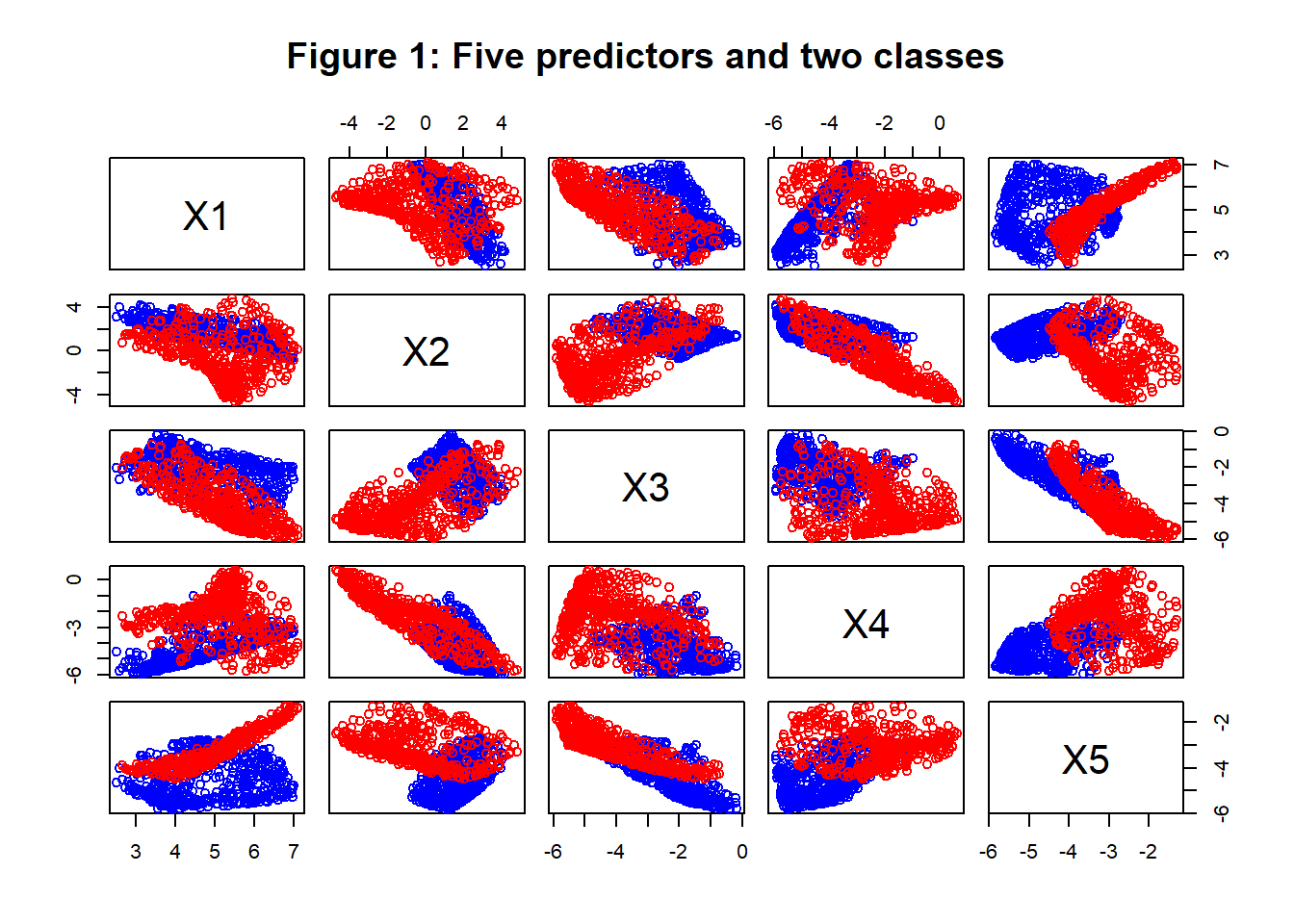
The five predictors for this example were generated using a three layer neural network with a (3, 6, 5) architecture and randomly generated weights and biases. Using three independent random uniform (-0.5, 0.5) variables for the inputs, a sample of size n=500 was generated with one set of random weights and biases and a second sample of n=500 was generated with a different set of random parameters.
Figure 1 shows the distribution of the 5 predictors in the two classes. The values of the predictors for class Y=0 are shown in blue and those for class Y=1 are shown in red.
A logistic regression model
Logistic regression provides a useful baseline analysis for comparison with any binary classification neural network. Table 1 gives the logistic regression coefficients for the data in figure 1 as provided by R’s glm() function. The coefficients show, for example, that the logit of the probability of being red (class 1) is larger when X5 is large, which agrees with the pattern in figure 1.
| Table 1: Logistic regression coefficients | |||
| term | estimate | std.error | p.value |
|---|---|---|---|
| (Intercept) | 20.2217 | 2.0245 | 0.0000 |
| X1 | −1.1362 | 0.1440 | 0.0000 |
| X2 | −1.6688 | 0.2114 | 0.0000 |
| X3 | 0.6584 | 0.2268 | 0.0037 |
| X4 | −0.5906 | 0.1885 | 0.0017 |
| X5 | 3.3976 | 0.3800 | 0.0000 |
Using a threshold probability of 0.5 (logit of zero), the predicted probabilities can be converted into class assignments and the confusion matrix can be calculated. Table 2 gives this matrix and shows that logistic regression misclassifies 11.9% of the training data.
| Table 2: Logistic regression confusion matrix | ||
| True Class | Predicted Class | |
|---|---|---|
| 0 | 1 | |
| 0 | 451 | 49 |
| 1 | 70 | 430 |
Table 3 shows the measures of goodness of fit for the logistic regression as extracted by the glance() function from the broom package. The cross-entropy is minus the average log-likelihood, which in this case is -logLik/nobs = 0.266.
| Table 3: Logistic regression goodness of fit measures | |||||||
| null.deviance | df.null | logLik | AIC | BIC | deviance | df.residual | nobs |
|---|---|---|---|---|---|---|---|
| 1386.294 | 999 | -266.0948 | 544.1895 | 573.6361 | 532.1895 | 994 | 1000 |
A neural network model
As an example of a simple neural network, I tried the (5, 3, 1) architecture in which the output is the probability of being in class 1 and sigmoid functions were placed on the hidden and output layers. The model was fitted using the gradient descent algorithm run for 50,000 iterations with a fixed step length of 0.1. As I used the binary cross entropy loss, this analysis can be thought of as logistic regression with a more flexible function of the five predictors.
The fitting algorithm drove the neural network’s cross-entropy down to 0.053, much lower than for logistic regression. Using the same threshold probability of 0.5, the confusion matrix of the neural network given in table 4, shows a reduced misclassification rate of 1.6% in the training data.
| Table 4: Neural network confusion matrix | ||
| True Class | Predicted Class | |
|---|---|---|
| 0 | 1 | |
| 0 | 500 | 0 |
| 1 | 16 | 484 |
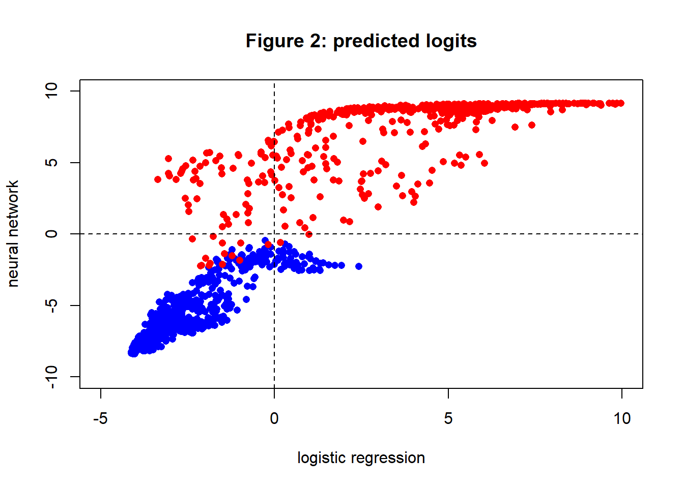
Figure 3 shows the predicted logit probabilities (log[p/(1-p)]) for the logistic regression and plotted against the logits of the neural network prediction. The separation of the points projected on to the neural network axis is clearly much better than the separation of the points projected onto the logistic regression axis. The points that are misclassified by one method and correctly classified by the other appear in the top left and bottom right sections of the plot. You will see that there is only one point that is correctly classified by logistic regression, but wrongly classified by the neural network. It is a red dot quite close to the intersection of the dashed threshold lines.
There is always a danger that performance on the training data will not accurately represent performance on future data, so a sample of test data with n=50,000 was generated using the process that created figure 1. The misclassification rates of the logistic and neural network models were calculated on the test data giving 10.7% for the logistic regression and 2.3% for the neural network; both are broadly in line with the performance of those models on the training data.
A simulated example of multi-class classification
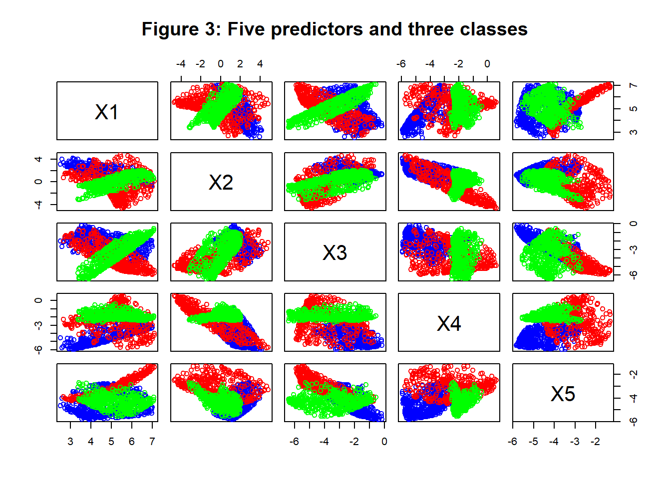
The method of data generation previously used to create the binary example was extended to add a third group of size 500 based on a new set of random weights and biases. The resulting predictors are shown in figure 3, with the new group plotted in green.
A logistic regression model
The simplest way to use logistic regression models to distinguish between three classes is first to use logistic regression to distinguish class 0 (blue) from the combination of classes 1 (red) and 2 (green) and then to fit a second logistic regression to distinguish class 1 (red) from class 2 (green) using the dataset without class 0. The two logistic regressions provide estimates of P(blue) and P(red|not blue), from which we can deduce that P(red)=P(red|not blue).P(not blue) or P(red)=P(red|not blue).[1-P(blue)] and of course, P(green)=1-P(blue)-P(red).
The coefficients of the logistic regression that distinguishes class 0 (blue) from the remainder are given in Table 5
| Table 5: Logistic regression of class 0 vs classes 1 and 2 combined | |||
| term | estimate | std.error | p.value |
|---|---|---|---|
| (Intercept) | −6.0767 | 0.9203 | 0.0000 |
| X1 | 0.0832 | 0.0840 | 0.3221 |
| X2 | 0.0955 | 0.0904 | 0.2908 |
| X3 | 0.5049 | 0.0965 | 0.0000 |
| X4 | −1.4382 | 0.0982 | 0.0000 |
| X5 | −0.4872 | 0.1299 | 0.0002 |
The coefficients of the logistic regression for distinguishing class 1 from class 2, excluding the data from class 0, are given in Table 6.
| Table 6: Logistic regression of class 1 vs class 2 | |||
| term | estimate | std.error | p.value |
|---|---|---|---|
| (Intercept) | 30.2544 | 2.5109 | 0.0000 |
| X1 | −1.5784 | 0.2109 | 0.0000 |
| X2 | 0.3835 | 0.1424 | 0.0071 |
| X3 | 0.4426 | 0.1255 | 0.0004 |
| X4 | −0.2254 | 0.1846 | 0.2220 |
| X5 | 5.6778 | 0.4211 | 0.0000 |
Combining the predictions from the two models we can estimate the probabilities of class membership for each of the three classes and assigning each item to the class with the largest probability gives the confusion matrix, which is shown in Table 7.
| Table 7: Three class logistic regression confusion matrix | |||
| True Class | Predicted Class | ||
|---|---|---|---|
| 0 | 1 | 2 | |
| 0 | 391 | 80 | 29 |
| 1 | 71 | 404 | 25 |
| 2 | 0 | 62 | 438 |
Overall 17.8% are misclassified by the pair of logistic regression models.
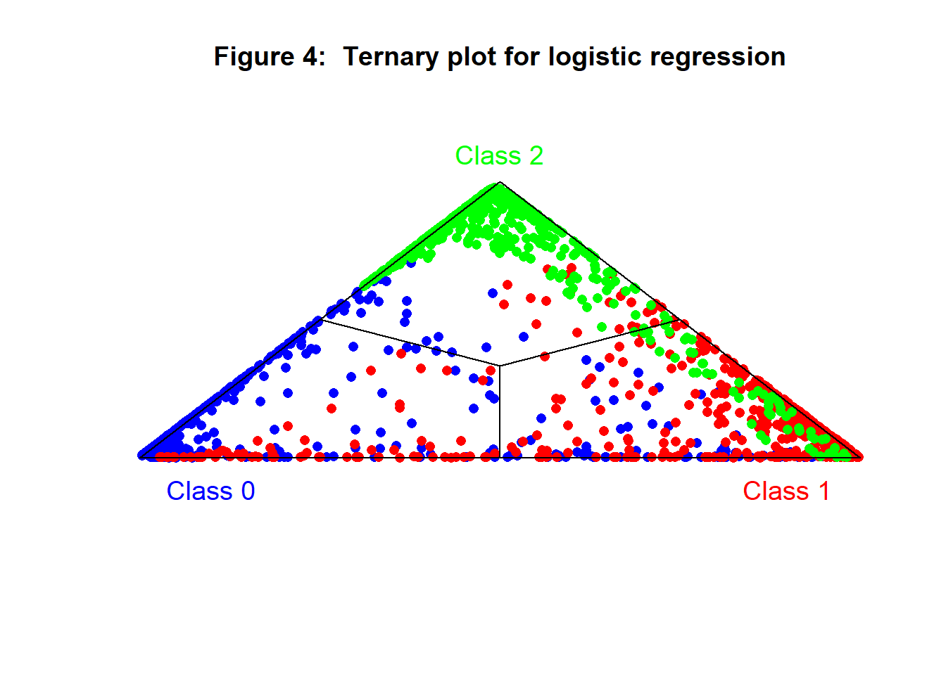
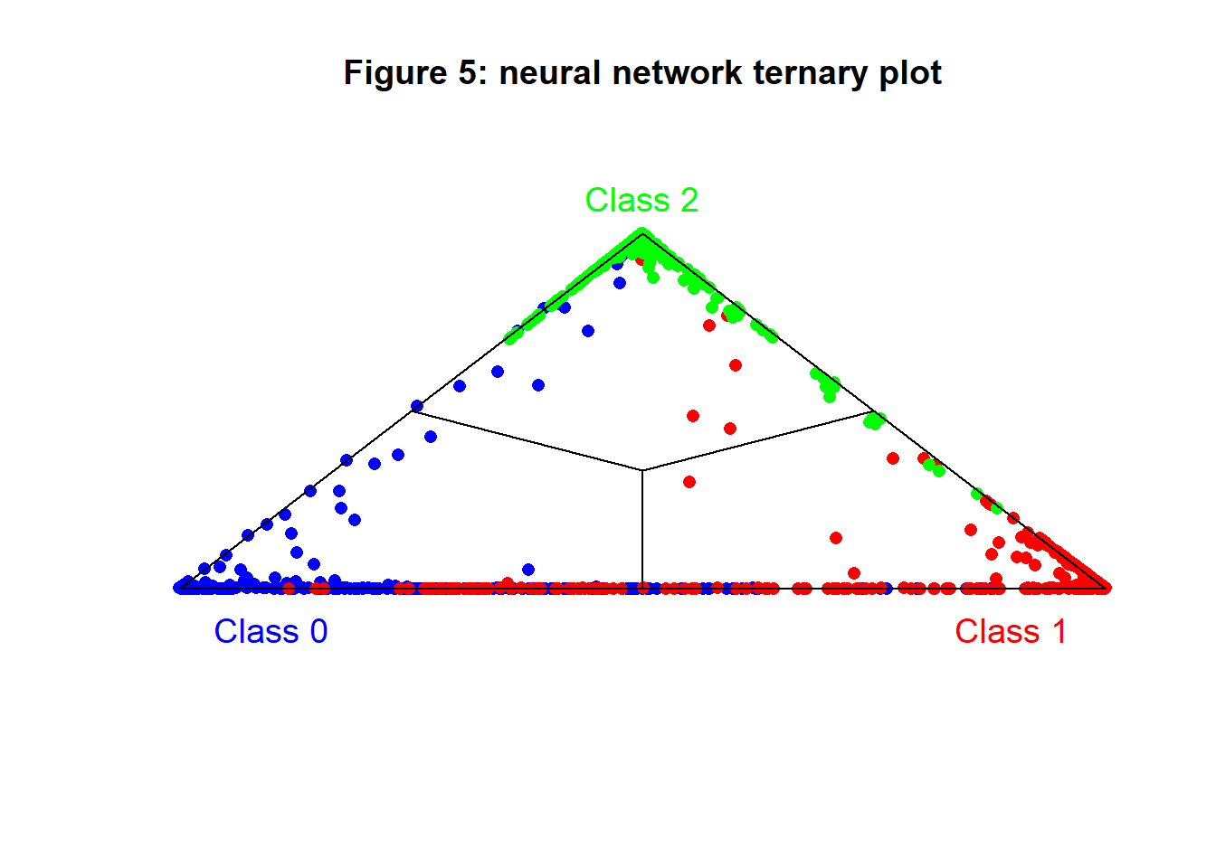
A neat way to show three proportions or percentages is in a ternary plot. This plot is easy to understand, but quite difficult to explain. If you are interested in the detail, you will find it on Wikipedia (https://en.wikipedia.org/wiki/Ternary_plot). Essentially the plot takes the form of a triangle with each class assigned to one of the corners. The points are plotted so that the greater the probability of being in that class, the closer the points are to that corner. When class membership is certain the point is plotted exactly on the appropriate corner and if the probabilities where (1/3, 1/3, 1/3) the point would be plotted in the centre of the triangle.
Figure 6 shows a ternary plot of the three predicted probabilities from the pair of logistic regressions. Ideally, the blue points should cluster in the bottom left corner, the red points in the bottom right corner and the green points at the apex. Where points are misplaced the item would be misclassified by this model. The plot shows, for example, that green points are never misclassified as coming from the blue class.
A neural network model
For the neural network analysis, the output layer has three values, one probability for each class and the observed classes, y, are coded (1, 0, 0) for class 0, (0, 1, 0) for class 1 and (0, 0, 1) for class 3.
I chose a (5, 3, 3) architecture for the neural network with a sigmoid activation on the hidden layer and softmax activation on the output layer. The weights and biases were obtained by minimising the multi-class cross entropy.
The confusion matrix for this neural network is given in Table 8.
| Table 8: 3-Class neural network confusion matrix | |||
| True Class | Predicted Class | ||
|---|---|---|---|
| 0 | 1 | 2 | |
| 0 | 458 | 28 | 14 |
| 1 | 60 | 434 | 6 |
| 2 | 0 | 9 | 491 |
Only 7.8% of the training data are misclassified by the neural network.
Figure 5 shows the ternary plot for the neural network. Notice how the neural network pulls the points towards the triangular frame of the plot. Very few points have an uncertain classification.
Cirrhosis
This dataset comes from kaggle’s playground competitions, which all use small to medium sized sets of tabular data to test machine learning skills (https://www.kaggle.com/competitions/playground-series-s3e26/overview). This particular dataset is based on original data from a Mayo Clinic study of primary biliary cirrhosis (PBC) carried out between 1974 and 1984 (https://www.kaggle.com/datasets/joebeachcapital/cirrhosis-patient-survival-prediction).
The outcomes of the patients were classified as died, given a liver transplant and censored, where censored means that at the end of the follow up period the patient was alive and had not yet had a transplant. The training set for this study is relatively small and consists of just 7905 patients, of whom 4965 were censored, 275 had had a transplant and 2665 had died.
The predictors for this study included 6 binary (yes/no) features, 9 continuous blood measurements, disease stage (1 to 4), age and the number of days in the study. Prior to analysis, I transformed the data as follows,
- age was converted to age in years
- days in the study was converted to years in the study
- all binary predictors were coded as 0/1
- stage was coded as 3 dummy 0/1 variables, representing stages 1, 2 and 3
- all continuous biological measurements were log10 transformed
- the response classes were one-hot encoded as sets of three 0/1 variables
For the following analyses, the 7905 patients were randomly divided into a training set of size 5000 and a test set of size 2905.
Logistic regression of the cirrhosis data
Table 8 shows the logistic regression coefficients for identifying those patients who died (as opposed to those who were either transplanted or censored) in the training set of size 5,000. Patients who die tend to be in the study for a shorter period of time (they die), they tend to be older, to be male, to be in stage 4 and to have high levels of Bilirubin and Prothrombin. Bilirubin is a product of the break down of red blood cells, a healthy liver will remove most bilirubin and keep the blood levels low, so I high level of bilirubin is indicative of liver disease.
| Table 9: Logistic regression coefficients for predicting death | |||
| term | estimate | std.error | p.value |
|---|---|---|---|
| (Intercept) | −21.6754 | 2.0404 | 0.0000 |
| N_Years | −0.0602 | 0.0151 | 0.0001 |
| Age | 0.0307 | 0.0041 | 0.0000 |
| Sex | 0.4000 | 0.1428 | 0.0051 |
| Drug | 0.2162 | 0.0813 | 0.0078 |
| Ascites | −0.0733 | 0.3121 | 0.8142 |
| Hepatomegaly | 0.4748 | 0.0967 | 0.0000 |
| Spiders | 0.3012 | 0.0942 | 0.0014 |
| Edema | 1.9310 | 0.4288 | 0.0000 |
| Stage1 | −1.1241 | 0.2417 | 0.0000 |
| Stage2 | −0.6909 | 0.1270 | 0.0000 |
| Stage3 | −0.6040 | 0.0967 | 0.0000 |
| Bilirubin | 1.5773 | 0.1350 | 0.0000 |
| Cholesterol | −0.0255 | 0.2733 | 0.9256 |
| Albumin | −3.1679 | 1.0352 | 0.0022 |
| Copper | 0.6981 | 0.1459 | 0.0000 |
| SGOT | 1.1781 | 0.2746 | 0.0000 |
| Alk_Phos | 0.6187 | 0.1431 | 0.0000 |
| Tryglicerides | 0.7036 | 0.2659 | 0.0081 |
| Platelets | −0.8334 | 0.2712 | 0.0021 |
| Prothrombin | 15.5841 | 1.4300 | 0.0000 |
The second logistic regression contrasts transplanted and non-transplanted patients amongst those who do not die. Transplants tend to be given to patients who are younger, but more seriously ill.
| Table 10: Logistic regression coefficients for predicting a transplant in patients who did not die | |||
| term | estimate | std.error | p.value |
|---|---|---|---|
| (Intercept) | −11.3233 | 4.4321 | 0.0106 |
| N_Years | −0.2227 | 0.0417 | 0.0000 |
| Age | −0.0561 | 0.0089 | 0.0000 |
| Sex | 0.1683 | 0.3257 | 0.6054 |
| Drug | 0.7917 | 0.1781 | 0.0000 |
| Ascites | 0.3316 | 0.7430 | 0.6554 |
| Hepatomegaly | 0.0922 | 0.2073 | 0.6567 |
| Spiders | 0.0022 | 0.2149 | 0.9920 |
| Edema | −14.5835 | 528.5210 | 0.9780 |
| Stage1 | −1.1402 | 0.5561 | 0.0403 |
| Stage2 | −0.6375 | 0.2767 | 0.0212 |
| Stage3 | −0.1885 | 0.2124 | 0.3748 |
| Bilirubin | 1.8086 | 0.2901 | 0.0000 |
| Cholesterol | −1.3260 | 0.5956 | 0.0260 |
| Albumin | 2.0729 | 2.4736 | 0.4020 |
| Copper | 1.2277 | 0.3435 | 0.0004 |
| SGOT | 0.9122 | 0.6128 | 0.1366 |
| Alk_Phos | 0.4470 | 0.3335 | 0.1801 |
| Tryglicerides | 0.4767 | 0.5702 | 0.4031 |
| Platelets | 1.0148 | 0.6502 | 0.1186 |
| Prothrombin | 4.9424 | 3.1815 | 0.1203 |
Combining the predictions from the two models on the test set of 2905 patients, gives the predicted probabilities for all three classes and assigning each patient to the class with the largest probability enables the test confusion matrix to be calculated; it is shown in Table 11. Overall 20.0% are misclassified and there is an obvious problem in identifying the patients who had had a transplant.
| Table 11: 3-Class logistic regression confusion matrix | |||
| True Class | Predicted Class | ||
|---|---|---|---|
| censor | transplant | death | |
| censor | 1642 | 0 | 175 |
| transplant | 57 | 0 | 49 |
| death | 309 | 0 | 673 |
The test 3-class cross-entropy loss for this model is 0.528.
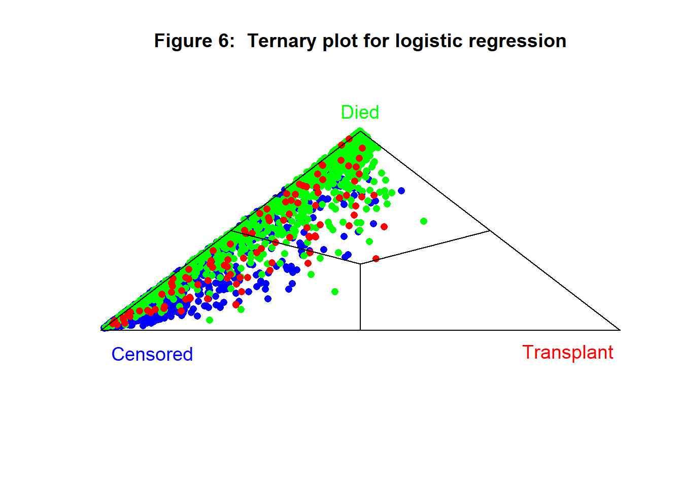
The ternary plot for the test sample is shown in figure 6, it confirms the generally poor performance of the model and the particular difficulty of identifying the transplant patients.
A Neural network model
The object of this exercise is to learn about neural networks, it is not about winning a kaggle competition. So rather than jumping in with a giant model, let’s stop and consider the characteristics of the challenge before us. Here are what I take to be the key elements,
- the training dataset is small, just 5,000 patients
- the transplant class is relatively uncommon, around 3% of the training data
- there are 20 predictors of which 9 are binary
- there are many important predictors that are not available to us, so it will be difficult to distinguish between the three classes
- a few of the predictors that we do have are not particularly informative
There are two ways that we could use a neural network in the analysis
- a single 3-class neural network that classifies the three classes in one model.
- as with the logistic regression, we could develop two neural networks, say, one of dead vs alive and a second model of transplant vs censored amongst survivors.
A single Neural Network
Let’s start with the 3-class neural network and consider what architecture we might use. The network cannot be too large or else the estimates of the weights and biases will become unstable. Regularisation could be used to counter this problem, but as yet I have not discussed regularisation in these posts so I want to avoid using it.
Without regularisation, a conservative guide is that 25 observations are needed for each model parameter, so, given that we have a training set of size 5,000, the neural network can have up to 5000/25=200 parameters. A neural network with architecture (20, h, 3) will have 24h+3 parameters, so the hidden layer can have a maximum of 8 nodes.
I used a (20, 8, 3) architecture with a zero-centred sigmoid activation function for the hidden layer and softmax activation on the output layer. The data were robustly scaled to lie in the range -0.5 to +0.5 and gradient descent with a step size of 0.1 was run for 30,000 iterations.
Figure 7 shows the loss reduction
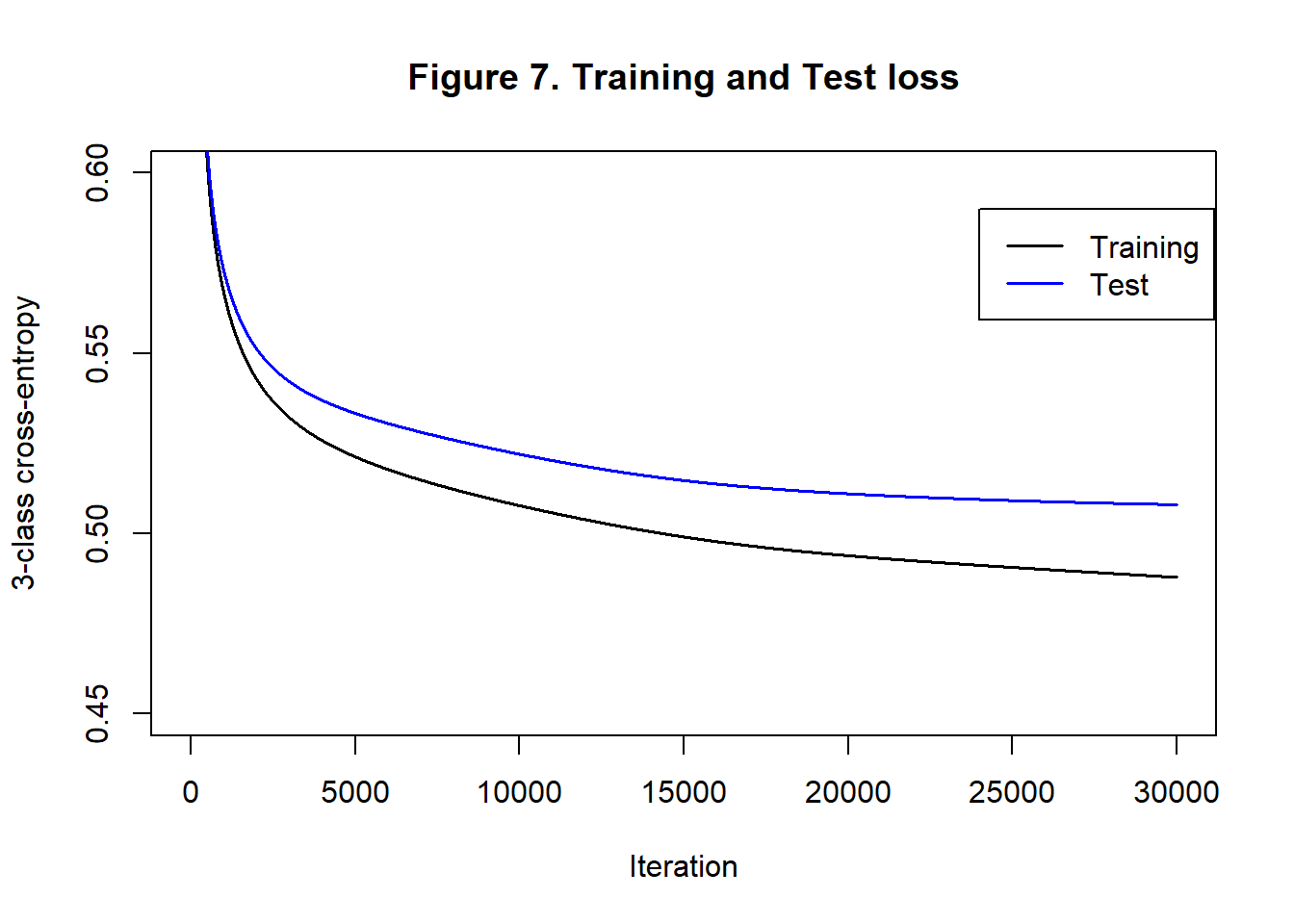
The training cross-entropy loss is reduced to 0.488 and the corresponding test loss is 0.508, not much better than logistic regression. As a check, I continued the algorithm for more iterations, but the test loss did not drop much further and after 80,000 iterations it started to increase. The confusion matrix shows that 20.3% of the test sample are misclassified by a largest probability rule, slightly worse than logistic regression.
| Table 12: Single Neural Network confusion matrix | |||
| True Class | Predicted Class | ||
|---|---|---|---|
| censor | transplant | death | |
| censor | 1619 | 0 | 198 |
| transplant | 51 | 0 | 55 |
| death | 285 | 0 | 697 |
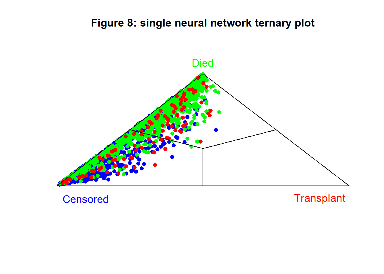
Figures 8 shows the class probabilities of the test sample in a ternary plot. Classification is as bad as it was with the logistic regression models.
A pair of neural networks
Suppose that we use a (20, h1, 1) neural network to distinguish dead from alive and a (20, h2, 1) neural network to distinguish transplants from survivors (censored) in those that do not die. In total, we will use 22(h1+h2)+2 parameters and if we keep to my guideline of 25 observations per parameter h1+h2 can be 9. The second model will not use the patients who die, so will only have 3317 observations, suggesting h2 can be up to 6. I opted for h2=4 and h1=5.
For both models, I used a zero-centred sigmoid activation function for the hidden layer and a sigmoid activation on the output layer. The data were robustly scaled to lie in the range -0.5 to +0.5 and then gradient descent algorithm was run for 20,000 iterations with a step size of 0.1.
The confusion matrix in table 13 shows that 20% are misclassified.
| Table 13: Two Neural Network confusion matrix | |||
| True Class | Predicted Class | ||
|---|---|---|---|
| censor | transplant | death | |
| censor | 1615 | 0 | 202 |
| transplant | 52 | 0 | 54 |
| death | 272 | 0 | 710 |
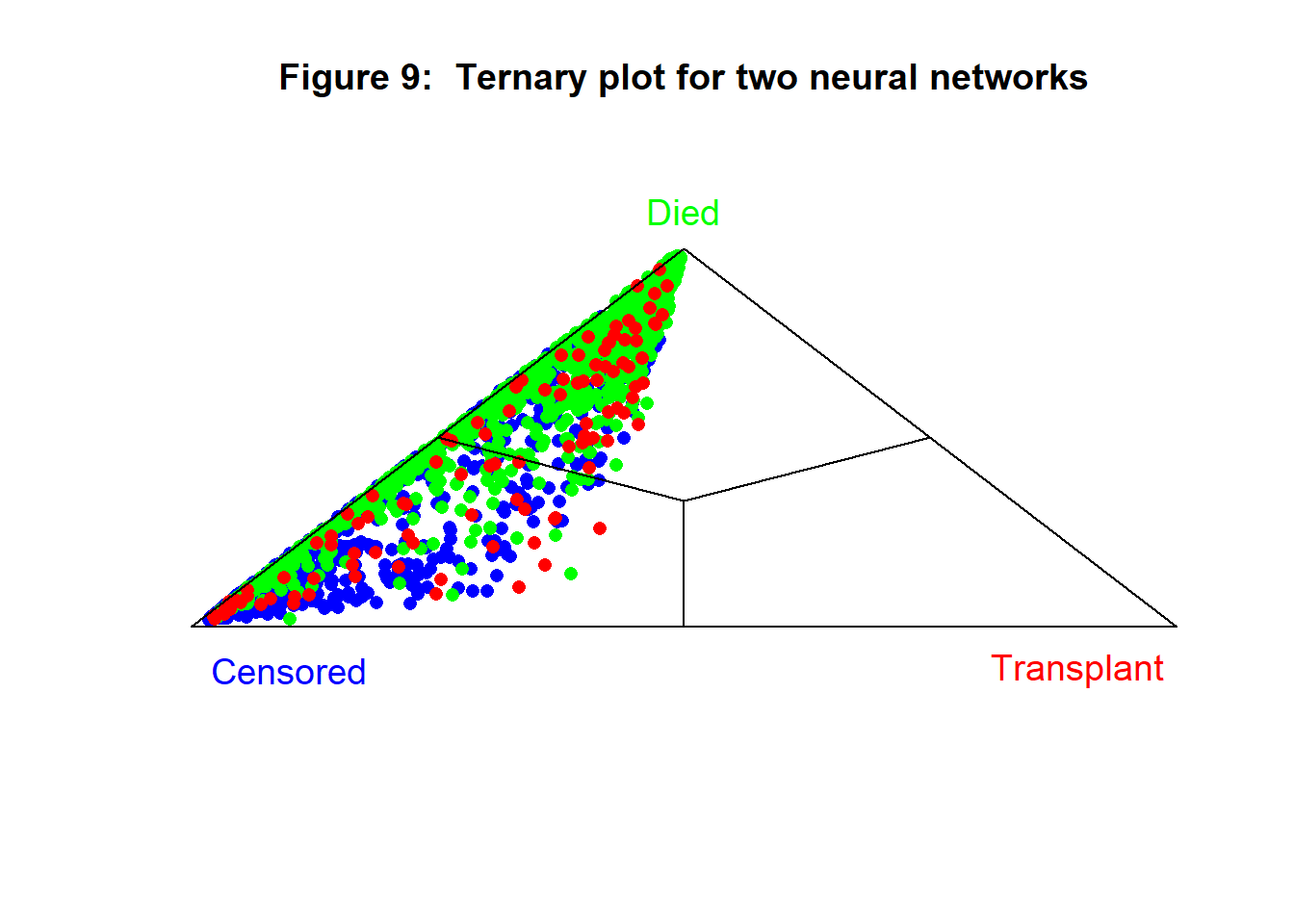
The 3-class cross-entropy for the combination of the two neural networks is 0.512 and the ternary plot is given in figure 9.
Thoughts on the Cirrhosis Analysis
The performance of these neural network models on the cirrhosis data is very disappointing, no better than logistic regression. Moreover, the leaderboard for the competition suggests that other machine learning models, i.e. XGBoost and its friends, can reduce the cross-entropy to 0.38. I need to understand why neural networks perform so badly. Here are some aspects of my cirrhosis analysis that might have impacted on the performance.
- Preprocessing: Perhaps there are derived features that are more informative; such as, albumin level divided by alkaline phosphatase or whatever. Alternatively, variable selection could be used to reduce the number of features. Other possibilities include, better transformations of the given features, data cleaning and the addition of the data from the original Mayo clinic study to increase the sample size. I am reluctant to use problem specific knowledge for fear that this will turn into a statistical analysis; my original aim was to use machine learning to find an automatic algorithm.
- Hyperparameter tuning: Perhaps there is a better set of weights and biases, but my algorithm failed to find it. I only tried one set of starting values, one step length and so on. My feeling is that tuning the algorithm might make a marginal difference, but it is not going to rescue these models, they are way off the pace.
- Ensembling: I only tried one split of the data, one random set of starting values and a very limited range of architectures. Perhaps averaging over multiple networks would improve performance.
- Imbalance: Much is made in the machine learning literature of the importance of imbalance and the cirrhosis data include the transplant class, which is much smaller than the other two classes and which is not identified at all by the neural network models. Perhaps, the poor performance is related to this imbalance.
- Trees are just better: Recently, a paper appeared on Arxiv entitled, Why do tree-based models still outperform deep learning on tabular data? (https://arxiv.org/abs/2207.08815). In that paper, the authors suggested possible reasons why neural networks perform poorly on some tabular datasets. Perhaps, that paper will suggest lines for future investigation. It would be good to know if there are aspects of the cirrhosis data that disadvantage neural networks, for example, the proportion of binary features, or the number of redundant features.
- The neural networks were just too small: Perhaps throwing computer power at the problem would enable me to find a better neural network. My training set had a size of 5,000, so what about a neural network with 10,000 parameters? Before I can fit such large models, I will need to cover two further topics, regularisation and stochastic gradient descent. I might even need to parallelise my code, or switch to keras.
I’ll return to each of these possibilities in my next few posts and, periodically, I’ll return to the cirrhosis data and see if I can find a better neural network model.