Neural Networks: Cross-validation
Introduction
In this series of posts, I am investigating how best to use neural networks on tabular data by experimenting with small simulated datasets. So far, I have
- written R code for fitting a neural network by gradient descent
- used Rcpp to convert the R code to C for increased speed
- pictured gradient descent search paths
- used neural networks to simulate datasets for use in my experiments
- made some tentative first steps towards a workflow
In this post, I look at cross-validation, a technique that is the backbone of most machine learning workflows, but which is questionable on both theoretical and practical grounds. As you will see, my conclusion is that cross-validation should be used cautiously and with awareness of its limitations. This is an opinionated post, so be prepared to disagree. If you are a fan of cross-validation, you might like to read the conclusions at the end of the post before deciding whether to wade through the details.
Models and algorithms
My background is in traditional statistics where a clear distinction is made between a model and a fitting algorithm, but too often for my taste, this distinction is blurred in machine learning . The fitting algorithm is a machine for generating models from training data, it is not itself a model. Models take in predictors (i.e. features or Xs) and output a prediction of the response. This distinction is crucial when calculating performance measures, you always need to ask yourself whether you are trying to measure the performance of a model, or the performance of an algorithm. In this post, I want to ask, what does cross-validation (CV) measure? and, is it a good basis for decision making?
Models and algorithms are assessed in the context of a particular source of data; a model might perform well with one type of data and badly with another. The most important measure of the performance of a model is its expected loss on new data from that source. This is the measure that I employed in my post on search paths. Unfortunately, outside of simulation studies, it is highly unlikely that sufficient test data will exist to enable the expected loss to be estimated with any accuracy.
The most important measure of a fitting algorithm is the expected loss of the set of models that are generated when training data are randomly sampled from the data source of interest. When judging the algorithm, you use the average of the expected losses of all of the models that the algorithm might generate, whereas when judging a model, you are interested in the expected loss of that particular model.
Resampling methods, of which cross-validation is one, compensate for not having a ready supply of test data by taking repeated samples from the training data. These methods usually have high variance, which makes them rather imprecise; what is worse, it is not obvious which type of loss they estimate.
Data Sources
Here is a list of some types of data that might be available to a data analysis.
Training data: the data used to fit the model
Validation data: data that are independent of the training data but from the same source. Used for model selection or tuning of the fitting algorithm
Test data: a second set of independent data from exactly the same source as the training data. Used for estimating the expected loss
Target data: independent dataset(s) representative of the situation(s) in which the model is intended to be used
Feature sets: independent dataset(s) containing the predictors, but not the responses. Usually assumed to come from exactly the same source as the training data. The responses are either withheld as a test of model prediction, or they are yet to be collected, or perhaps they would be difficult or expensive to collect.
- never modify the analysis based on the test data
- never predict performance based on the validation data
Validation and test data can be created in simulation experiments, but otherwise they rarely exist in quantity. In the rare situations when real validation and/or test data are available, it is wise not to accept them unquestioningly. An important part of the data analysis workflow is to confirm their similarity to the training data.
The most common situation is to have training data and nothing else. When the training set is huge, a proportion of it can be reserved as a holdout sample for validation and/or testing, but if it is not huge, resampling is the only option.
Some notation
This section might, at first sight, seem a little pedantic, but it is important. Stick with it.
I want to refer to the actual training data and to other potential sets of training data, so I will use the subscript \(A\) to refer to what is Actually observed. This means that \(T_A=(X_A, Y_A)\) refers to the actual training data, to which I apply my favourite algorithm, F, (F as algorithms are Functions that generate models from data and A has already been claimed). F applied to \(T_A\) leads me to a model \(M_A\) with parameters \(\theta_A\).
Given any set of features, X, the fitted model, \(M_A\), will predict the responses by, \(M_A(X)\). My chosen loss function measures the size of the errors when observed responses are contrasted with predicted responses, so the actual training loss is \(L_A(M_A) = Loss(Y_A, M_A(X_A))\).
I am interested in how well \(M_A\) will perform in the future, so let’s imagine a large set of test data \(T_t\) (t for test) drawn from the same source as \(T_A\). Performance on the new data will be measured by, \(L_t(M_A) = Loss(Y_t, M_A(X_t))\), that is to say it will compare the test responses, \(Y_t\), with the predictions made by model \(M_A\) when it is applied to \(X_t\). \(L_t(M_A)\) is an estimate of the expected loss of \(M_A\). It might seem obvious, but let me stress that \(L_t(M_A)\) is a measure of the quality of model \(M_A\) and it does not depend on the algorithm used to suggest \(M_A\).
Now let’s assess the algorithm F. F will have its own parameters, such as the step length, the number of iterations and so on. Let’s assume that we have decided on a fixed set of algorithmic parameters, so that F is completely defined.
Imagine applying algorithm F to \(m\) training datasets, \(T_i \ \ i=1,\dots,m\), (i for imagined) of the same size as \(T_A\) and from the same source. Each of these datasets leads to a model \(M_i\), with parameters \(\theta_i\) and a new test loss, \(L_t(M_i) = Loss(Y_t, M_i(X_t))\). The performance of this algorithm on datasets of this size is captured by the average of these test losses, \[ L_F = \frac{1}{m} \sum_{i=1}^m L_t(M_i) = \frac{1}{m} \sum_{i=1}^m Loss(Y_t, M_i(X_t)) \]
\(L_F\) averages the performance of models created by using F on different training sets and it will be small when the algorithm produces good models when applied to a range of training data. It does not depend on \(M_A\), so it cannot be a direct measure of the quality of \(M_A\).
When you want to judge the quality of a model, you should use \(L_t(M_A)\) and when you want to judge the quality of an algorithm, you should use \(L_F\). For problems such as model selection and model assessment, \(L_F\) is almost irrelevant. The only connection between \(L_F\) and the assessment of \(M_A\) comes from the argument; F is a good algorithm, I used F to get \(M_A\), so \(M_A\) is probably a good model.
This distinction between \(L_t(M_A)\) and \(L_F\) matters for cross-validation (CV), because CV splits the training data into K parts called folds. In turn, each fold, f, is used as a holdout sample and F refits the model to the remaining data, \(\sim f\). The cross-validated loss is the average of the loss estimates from the K holdout samples. \[ L_{CV} = \frac{1}{K} \sum_{f=1}^K L_f(M_{\sim f}) = \frac{1}{K} \sum_{f=1}^K Loss(Y_{f}, M_{\sim f}(X_{f})) \] The form of \(L_{CV}\) resembles that of \(L_F\). \(L_{CV}\) is an imprecise estimate that averages different models generated by F when it is applied to datasets that are not independent. Averaging over different models suggests that it might be measuring \(L_F\), but because of the lack of independence, all K models will be similar to \(M_A\), so it might be close to \(L_t(M_A)\). There again. perhaps, it will not be close to either.
Cross-validation is itself a type of function that takes \(F\), \(T_A\) and a random split into folds, \(s\), and outputs a loss. We might write it as, \[ L_{CV} = CV(F, T_A, s) \] Since \(M_A = F(T_A)\) we might wonder if cross-validation can be performed using \(M_A\), as in CV(\(M_A\), s), but this is clearly impossible because we would have no data to cross-validate. What about, CV(\(M_A\), \(T_A\), s)? This too is impossible, because we need F to refit the model K times. The conclusion is important for the way that we should think about cross-validation.
There is no such thing as the cross-validation of a model.
When the algorithm is the target
There are situations in which we actually want to compare algorithms rather than models, most importantly when tuning hyperparameters, i.e. parameters of the fitting algorithm. However, even when tuning hyperparameters there is some ambiguity; we could be interested in creating an algorithm that works well for a typical set of training data from this source (low \(L_F\)), or more likely, we might want to optimise the performance of F when it is applied to the actual training data (low \(L_t(M_A)\)). It is when an algorithm is judged by how well it performs on the actual training data that the distinction between algorithm and model gets blurred.
There are two comparisons that we could make based on cross-validation that look deceptively like model comparison. Firstly, we have the comparison of the same algorithm applied to two different sets of training data, \[ CV(F, T_A, s) \ \ vs. \ \ CV(F, T_B, s) \] This looks like, but isn’t, a comparison of models \(M_A=F(T_A)\) and \(M_B=F(T_B)\). Secondly, we have the comparison of two different algorithms applied to the same data, \[ CV(F_1, T_A, s) \ \ vs. \ \ CV(F_2, T_A, s) \] This looks like, but isn’t, a comparison of models \(M_1=F_1(T_A)\) and \(M_2=F_2(T_A)\).
Hyperparameter tuning is usually concerned with the second of these possibilities. What we need to ask is, if I select my algorithm based on \(CV(F_1, T_A, s) \ \ vs. \ \ CV(F_2, T_A, s)\), will I make the same choice as I would have made from comparing \(L_t(M_1) \ \ vs \ \ L_t(M_2)\), i.e. will I choose the model with the best performance on future data. It is possible that the CV comparisons will lead to the best model, even if CV is a poor estimate of the test loss.
Hastie, Tibshirani and Friedman
When I first became interested in the connections between traditional statistics and machine learning I turned to Hastie, Tibshirani and Friedman’s (HTF) book “The Elements of Statistical Learning”. It is excellent and I always refer to it when I am confused or unsure.
HFT have an interesting chapter on “model assessment and selection” in which they discuss issues such as cross-validation. In that chapter, HTF finish by saying
“We conclude that estimation of test error for a particular training set (\(L_t(M_A)\)) is not easy in general, given just the data from that same training set (\(T_A\)). Instead, cross-validation and related methods may provide reasonable estimates of the expected error (\(L_F\)).”
The brackets are my additions that I inserted because HTF use a different notation.
As we will see, my simulations confirm that cross-validation is not a good measure of model performance, because it is only loosely related to \(L_t(M_A)\) and, although it does appear to be unbiased for \(L_F\), there are very few situations in which \(L_F\) is of any interest. HTF see the fact that cross-validation is unbiased for \(L_F\) as a positive, while I am more interested in the correlation between cross-validated loss and test loss, because that is what is usually needed for hyperparameter tuning.
Cross-validation
Cross-validation is a resampling method that divides the training data at random into K (usually K=5 or 10) equally sized subsamples called folds. In turn, each fold is reserved for validation and the model is fitted to the pooled data from the other K-1 folds. In this way, K measures of performance are created and their average is the CV estimate.
The simulation scenario
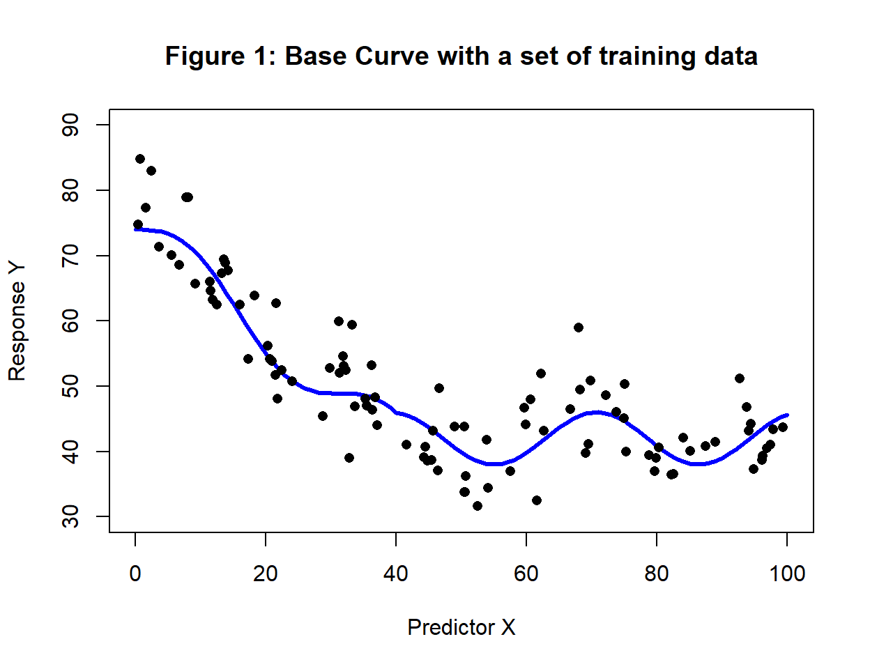
I generated a curve by adding a sin function to a linear trend with a break point at 40. The single predictor X was generated uniformly between 0 and 100 and the response was scaled to lie between about 30 and 80. A training set of size 100 was produced by adding Gaussian noise with a standard deviation of 5. A test set (\(T_t\)) with n=100,000 was used to estimate the expected loss.
Figure 1 shows the base curve together with a random set of training data (n=100).
CV for assessing models
The model family for my analysis of these data is a neural network with architecture (1, 6, 1) and a zero-centred sigmoid activation function. By (1, 6, 1) I mean, one input node, six hidden nodes in a single layer and one output node.
Since I want to start with the assessment of models, I must be careful to ensure that I use exactly the same algorithm for every simulation. My chosen algorithm, which I will call \(F_1\), is
- gradient descent
- step length fixed at 0.1 throughout
- exactly 1,000 iterations
- exactly the same starting values (randomly generated with a seed of 2308)
- robust scaling of the data as described in my post on workflow
The loss function used for measuring model performance will be the Root Mean Square Error (RMSE). The simulation of the data used a standard deviation of 5, so the test RMSE of a good, but not perfect, model will be slightly over 5.
It is an aside, but fully specifying the algorithm in advance is a good discipline. It helps avoid the bad practice of tweaking the analysis based on the results. Not only does such bad practice introduce selection bias, but it makes the workflow non-reproducible.
A single set of training data
Figure 2 shows the training data together with the curve fitted by algorithm \(F_1\). Presumably, the algorithm would need more iterations to find the finer structure in the data, but that need not concern us for the moment. Here, we simply want to measure the performance of the model represented by the green curve.
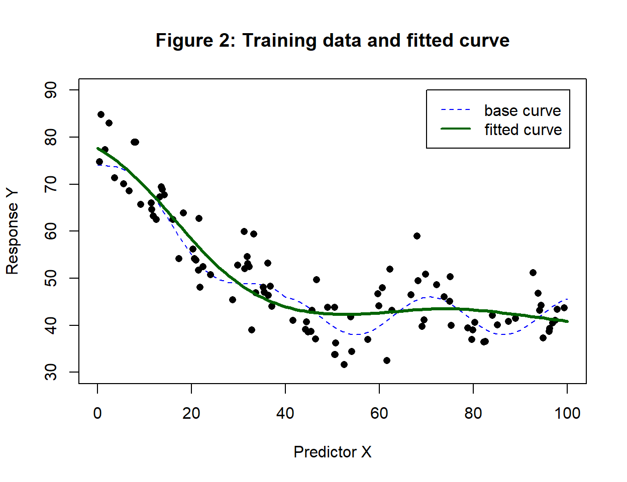
For these data, \(F_1\) gives weights and biases that define a model, (\(M_A\)), with a training loss (RMSE) of 5.29, a test (expected) loss of 5.59 and a 10-fold CV loss of 5.53.
Figure 3 shows the RMSEs from each fold. The training loss of the model fitted to 90% of the training data is on the x-axis and the validation error from the 10% holdout sample is on the y-axis. The horizontal dashed line corresponds to the cross-validation estimate and the vertical dashed line marks the training loss of the full training data. A regression line is shown in green.
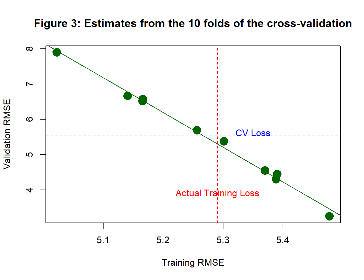
There are several points to note from figure 3.
- the fold-wise estimates (validation RMSEs) vary considerably ie. they have large variance
- there is a very strong negative correlation between the fold-wise training and validation losses
- the average of the fold-wise training RMSEs (5.27) is lower than the RMSE of the full training data (5.29)
- the average of the cross-validated losses (5.53) is quite close to the test loss(5.59)
The high variance in the fold-wise estimates means that we should not draw any firm conclusions from one example. We will need to simulate lots of sets of training data.
The negative correlation is understandable because a single response, y, that is randomly away from the fitted curve will either be in the training folds, in which case the training loss will increase, or it will be in the holdout sample, in which case the validation loss will increase and the training loss will correspondingly decrease.
The slight decrease in the average training loss is also understandable. In the cross-validation, the neural network only needs to fit to 90 observations instead of 100. An over-parameterised, flexible model ought to be able to reduce the training loss by more in a smaller sample.
Just what the cross-validation is estimating is much less clear. It looks like it might be the test loss, but the large variance means that it could be something else entirely. We will see shortly that the closeness of the cross-validation loss to the test loss seen in this example is unusual. Sometimes single simulations do throw up misleading results.
One approach that might at first sight seem attractive is to increase the number of folds, perhaps from 10 to 20. The average would then be taken over 20 estimates instead of 10. Unfortunately, each of those estimates would now be based on a holdout sample 5 observations instead of 10, so their variance would increase. There is clearly a trade-off between the number of estimates and the variance of those estimates. When other people have investigated this, they seem to agree that 10 folds is about the optimal number.
Another possible way of using CV is to create a regression estimate. In figure 3 the green line represents the regression of validation RMSE on training RMSE across the folds. The actual training loss meets this line when the validation RMSE is about 5.3. This estimate is specific to the actual training data and might be a better statistic to use for model comparison.
Finally, we need to keep in mind that CV might be susceptible to small sample bias. The pull of the training loss might well be stronger in small samples, so that although CV wants to estimate the test loss, it is only able to do so when the training set is large. I’ll consider sample size after I have looked at the current scenario.
Other splits
The division of the training data into K folds takes place at random, so the CV loss is based on one particular random split. Suppose I had used a different split, would the CV loss have changed? and if so, by how much?
To investigate this, I ran the cross-validation with 50 different splits of the same training data and got the results shown in figure 4.
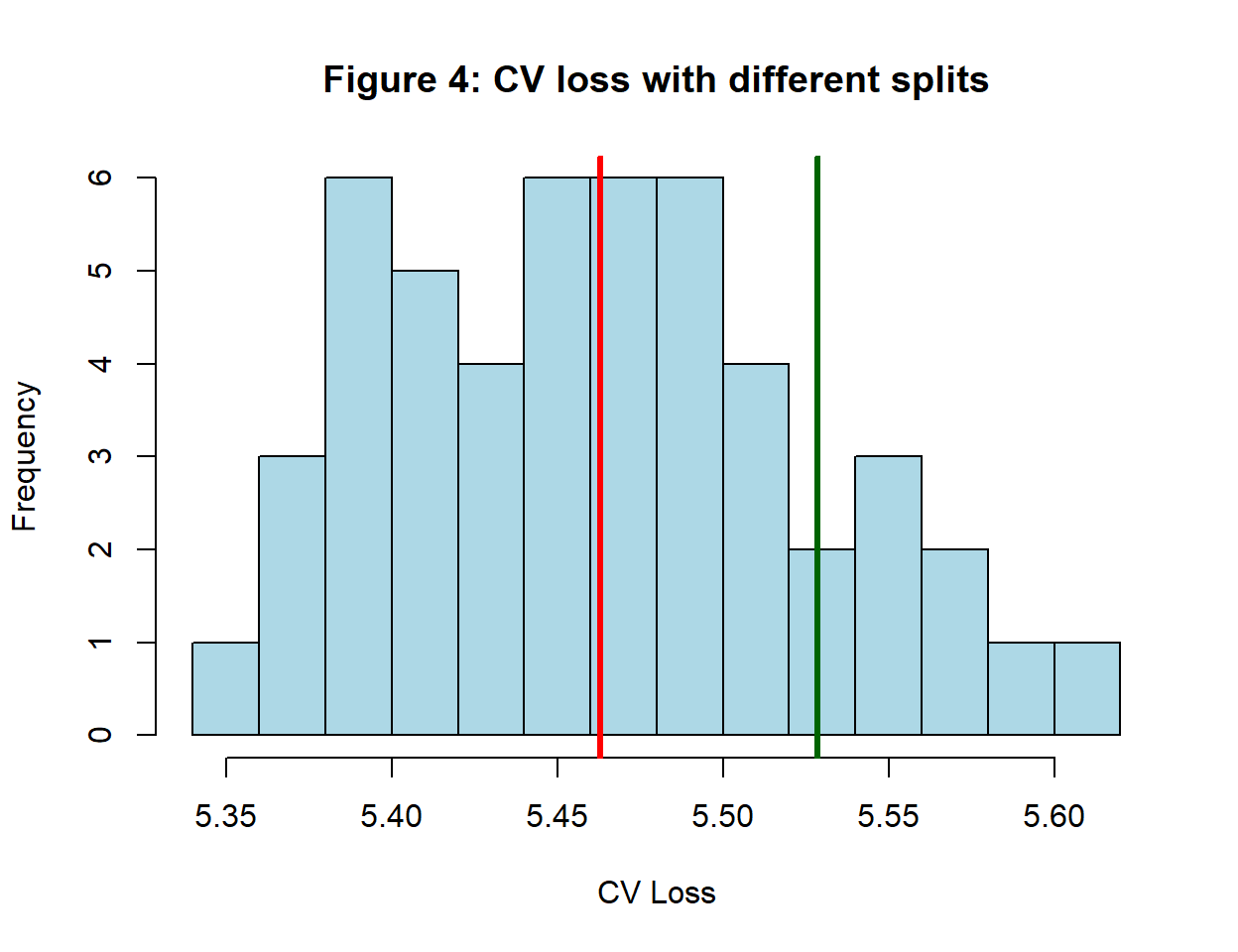
Clearly, we cannot place too much reliance on a single CV estimate; by chance, we might have obtained anything between 5.36 and 5.61. The mean of this distribution, shown in red, is 5.46, fairly close to the test loss of 5.59; another co-incidence? The CV loss for the split used in figure 3 is shown in green and confirms that that cross-validation was not typical.
50 sets of training data
In this section, \(F_1\) will be applied to 50 different sets of training data randomly drawn according to the method used to create figure 1. \(F_1\) will generate 50 models, one from each training set. There are several questions that we might ask,
- is the similarity between test loss and CV loss that we saw in the single simulation typical?
- which of these 50 models is best for predicting future data, i.e. which has the lowest test loss?
- how well does CV loss estimate the test loss of a particular model?
- how well does the average CV loss estimate the average test loss?
- is it sensible to choose between the 50 models based on the CV loss?
Figure 5 shows histograms of the training losses and test losses of the 50 models. The average training loss (5.38) is shown in red. 1,000 iterations is not many, so it is not surprising that the training loss of \(F_1\) rarely gets below the theoretically perfect RMSE of 5. The distribution of test losses has a theoretical lower limit of 5.0 due to the form of the simulation. The fact that the lowest test loss is 5.53 is further evidence that the models generated by the algorithm tend to underfit the data.
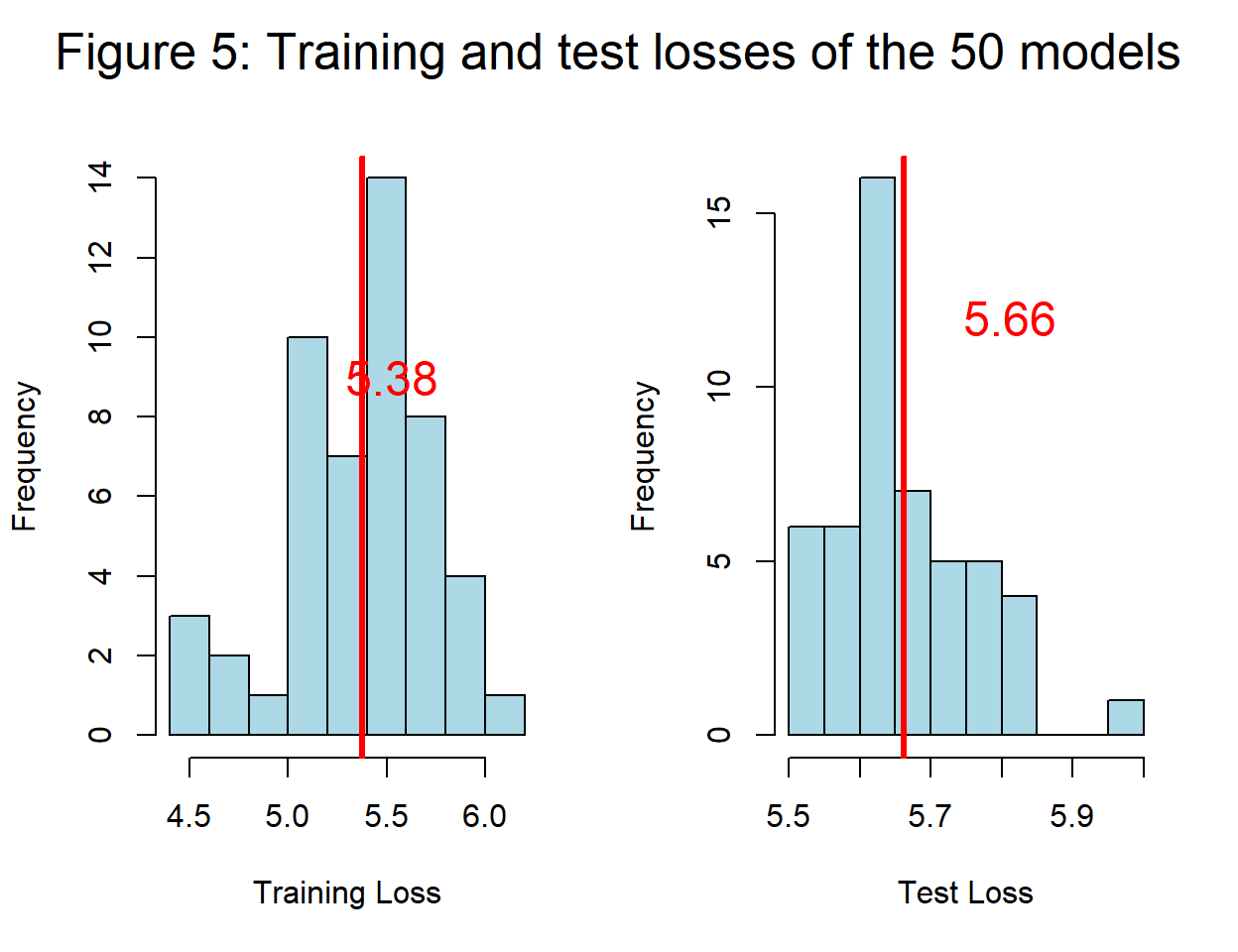
The average of the distribution of test losses, 5.66, is a summary measure of the performance of the algorithm on different training data from this source, i.e. it is an estimate of \(L_F\).
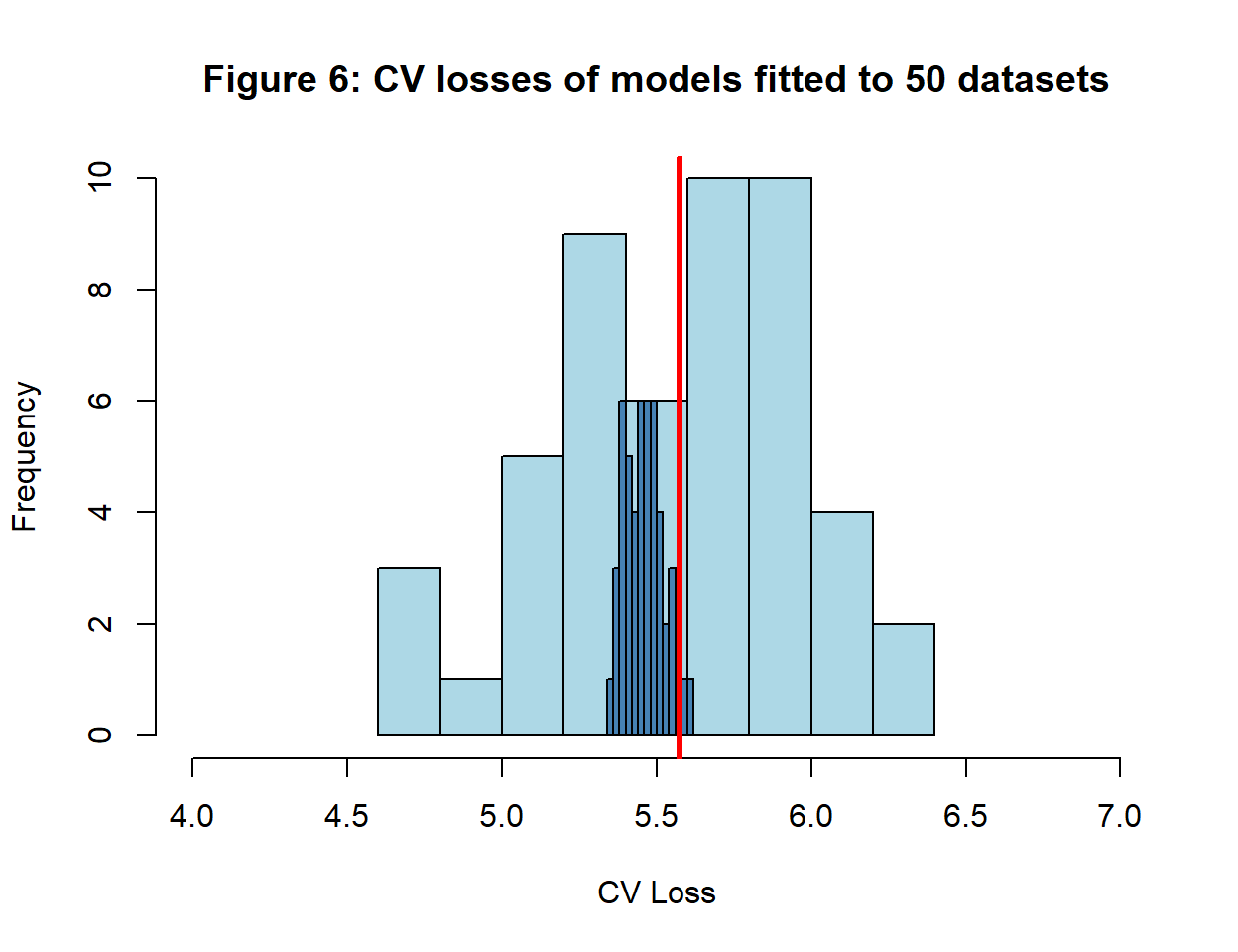
Each of the 50 training sets produces its own CV loss, which I calculated from a single random split into 10 folds. They are plotted in figure 6 with the average CV loss (5.57) in red; this average is very close to the average test loss. The super-imposed plot shows the variation between different splits of the same training data and is taken from figure 4.
The test losses vary between 5.53 and 5.96 while the CV losses vary between 4.65 and 6.34. The correlation between them is -0.292 and it would have been closer to zero if it were not for a single outlier. Figure 7 shows the relationship. The line represents equality between test and CV loss, it is NOT a regression line. CV loss is only loosely associated with the test loss, but the averages of the two losses are very similar as can be seen from the dashed lines that meet close to the line of equality.
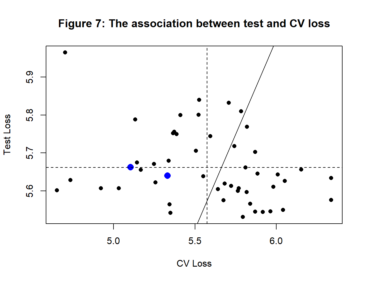
In figure 7, losses for two of the 50 models are highlighted in blue. It is clear that based on the smaller test loss, you would chose one model, and based on the smaller CV loss, you would choose the other. CV loss is neither a good estimate of the test loss of a single model nor is it a good basis for model comparison.
Bear in mind however, that this is a comparison of \(CV(F_1, T_A, s) \ vs. \ CV(F_1, T_B, s)\), i.e. the same algorithm applied to two random sets of training data. It is hard to think of any circumstances under which this comparison would be of practical importance. Applying \(F_1\) to different sets of training data is the basis of the calculation of \(L_F\), it is not designed to tell us anything about models.
The training losses come from the very data that we split for the CV and this creates a strong correlation (0.973) between training and CV losses. Figure 8 shows these two losses and how closely associated they are.
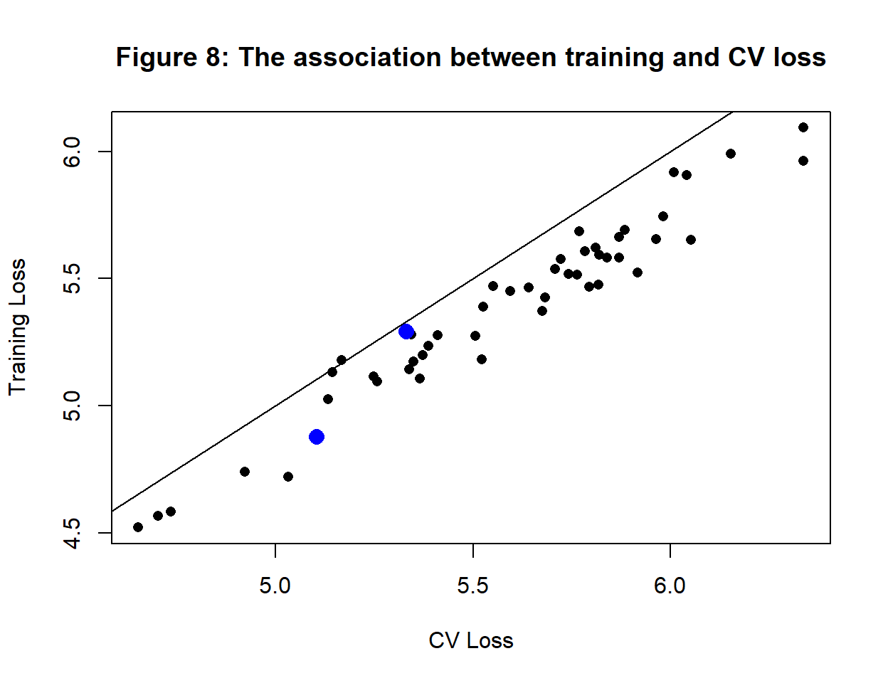
The same two models are highlighted in blue and now it is clear that the choice that you would make based on CV loss is the same as if you had used the training loss. Cross-validation consistently exceeds the training loss with a difference that averages 0.2. The CV loss is higher than the training loss and therefore closer to the test loss, but given the method, how could it be otherwise?
Larger Sample size
I mentioned the possibility that small sample bias might affect the CV loss. I investigated this by repeating the analysis based on \(F_1\) and 50 training sets of size n=400. Four times the sample size should reduce the spread by about a half. The plots within figure 8 correspond to figures 5, 6, 7 and 8.
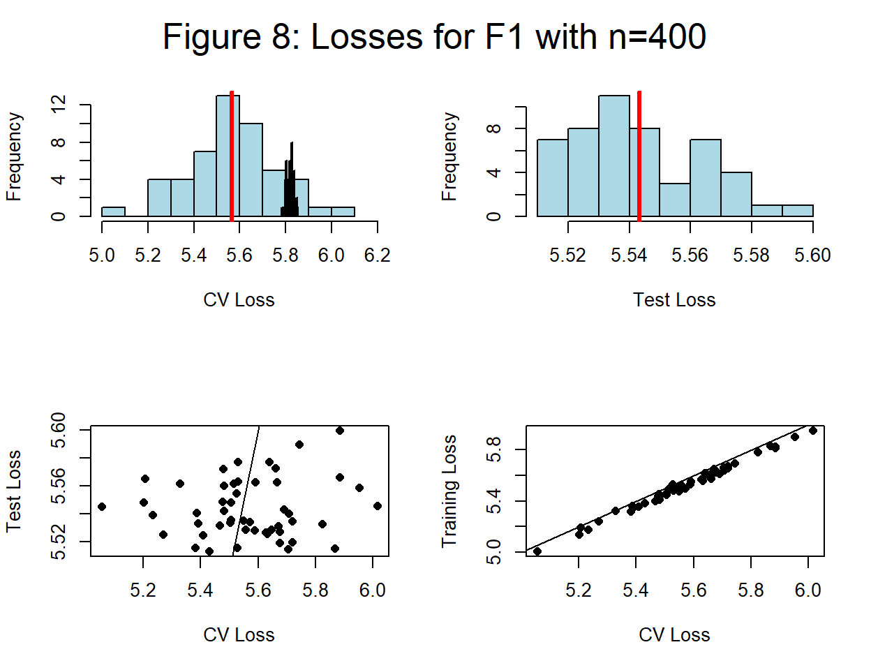
Several things are immediately obvious,
- the variances of all of the loss estimates are much smaller
- the average CV loss, 5.57, is quite close to the average test loss 5.54
- the correlation between the training loss and the CV loss is high (0.995)
- the correlation between the test loss and the CV loss is low (0.099)
With a larger training set the average CV loss remains close to the average test loss, but the correlation between the two is still low. This is consistent with HTF’s statement that the average CV loss estimates what I call \(L_F\), that is, it estimates the average test loss across all possible training datasets. However, being unbiased does not imply that test and CV loss will be correlated. CV loss is not a substitute for test loss when working with a single training set.
Conclusions about Model Assessment
If these simulation experiments are anything to go by, CV loss has a high variance and it correlates poorly with the test loss. In fact, the CV loss is highly correlated with the training loss. Use the CV loss for model selection and you are likely to reach the decision that you would have arrived at from the training loss, but not necessarily the “correct” decision as given by the test loss.
Increasing the size of the training set helps reduce the large variance of the CV loss and makes CV loss and test loss closer on average. However, agreement on average does not imply correlation, so you cannot use CV loss as a substitute for test loss when comparing two models generated by the same algorithm on different data.
Perhaps you are not interested in models generated by the same algorithm on different datasets, but if you are, things look bleak for cross-validation.
CV for assessing algorithms
In the previous simulations, I ran the gradient descent algorithm for exactly 1,000 iterations and called the algorithm \(F_1\). As an example of algorithmic change (hyperparameter tuning), I will re-analyse the same training data with the algorithm modified to run for 2,000 iterations; I call this algorithm \(F_2\). Initially, I revert to n=100.
Figure 10 shows a collection of plots based on \(F_2\) and n=100.
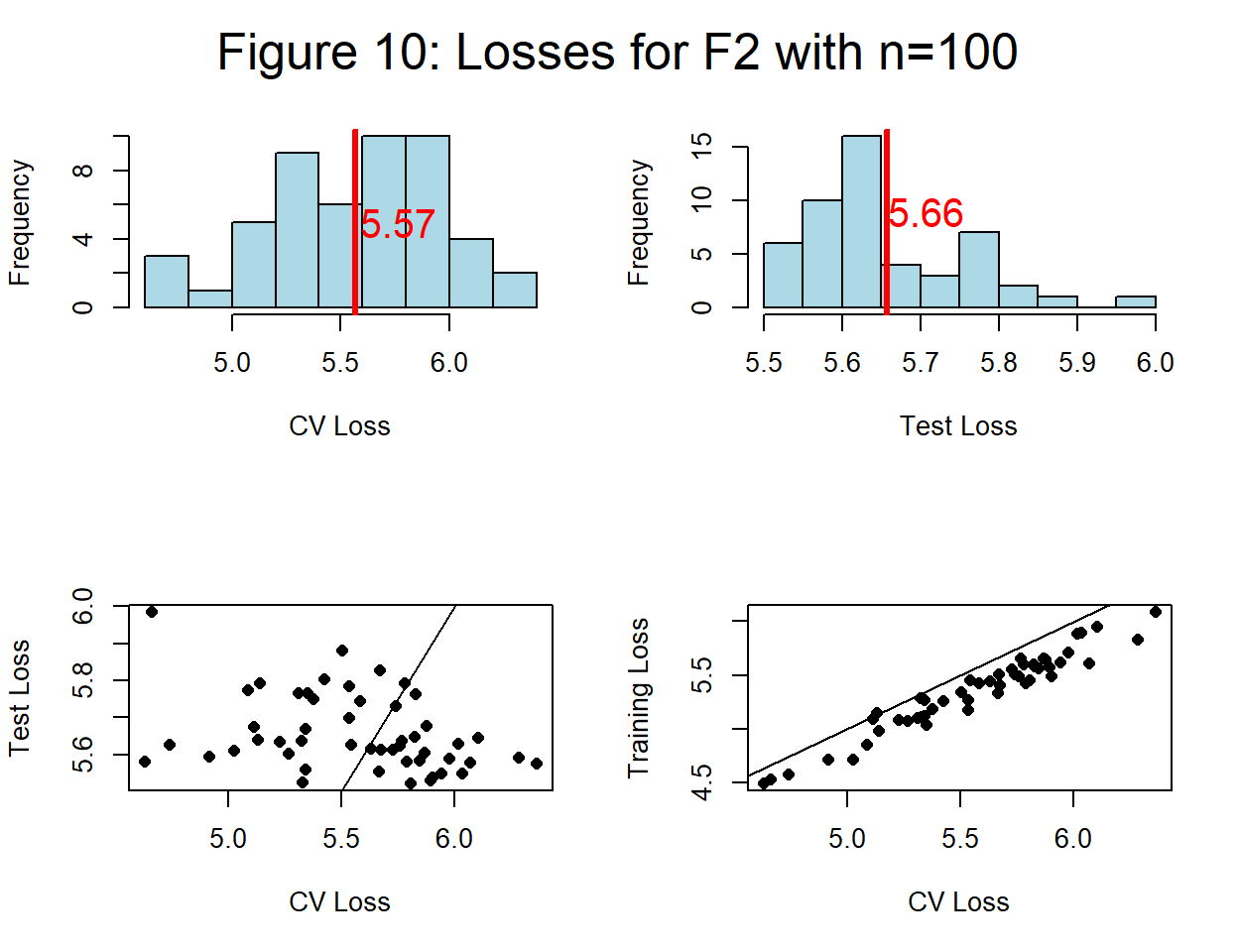
This plot has not compared the two algorithms, all that figure 10 demonstrates is that average CV agrees with average test loss, but for individual training sets there is little correlation. This holds whether the models come from \(F_1\) or \(F_2\).
Averaged over 50 training sets, CV and test losses agree but in reality, we will not have 50 training sets to average, so is it safe to base algorithmic choice on cross-validation of a single training set? Figure 11 tries to address the second question by plotting the differences between the test and CV losses of \(F_1\) and \(F_2\) for each training set.
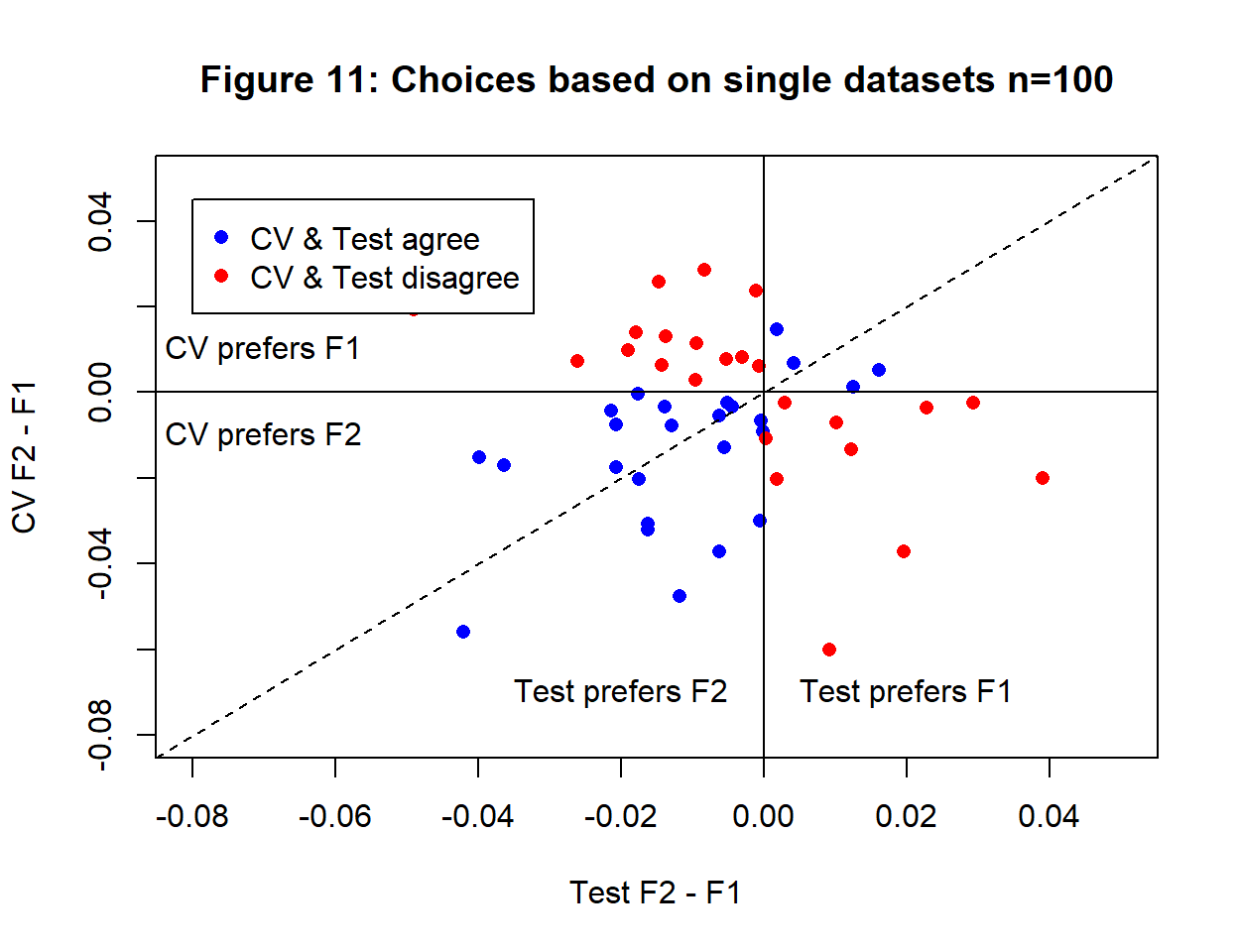
Based on the test loss, 15 datasets give better models after 1000 iterations and 35 give better models after 2000 iterations. If the “correct decision” is that suggested by the test loss then \(F_2\) is better most of the time.
The CV decision agrees with the test loss decision 25 times out of 50 (50%), which makes cross-validation no better than basing your hyperparameter tuning on spinning a coin. The correlation between test loss differences and CV loss diffences is only -0.057.
Figure 12 is similar to figure 11 but is based on training data with size n=400.
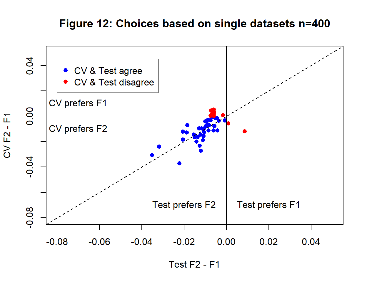
The variances have reduced and it is now clearer that \(F_2\) is the better algorithm and most (80%) of the time the CV and test criteria agree. The correlation between the differences is also higher (0.666). For clear differences between algorithms, as we have here, CV and test agree, but finer differences and smaller sample sizes will lead to many more disagreements.
I consider the results of the simulation with n=400 to be quite encouraging. Not many people would use cross-validation with a sample size as low as 100. Conversely, a (1, 6, 1) neural network only has 19 parameters and it is hard to say how large a sample size would be needed for a more complex model. It seems that, even though CV gives a poor measure of model performance, hyperparameter choices based on the cross-validation of a ‘reasonable sized’ training set look as if they might be useful.
Many algorithms
In this simulation, I compare many different algorithms. I run the gradient descent algorithm as before but for 1,000 to 20,000 iterations in steps of 1,000. This is a total of 20 algorithms and I want to pick the one with the best performance. The analysis is repeated on 50 training sets and I ask whether CV will select the same algorithm (number of iterations) as the test loss.
Figure 13 illustrates the analysis using a single set of training data.
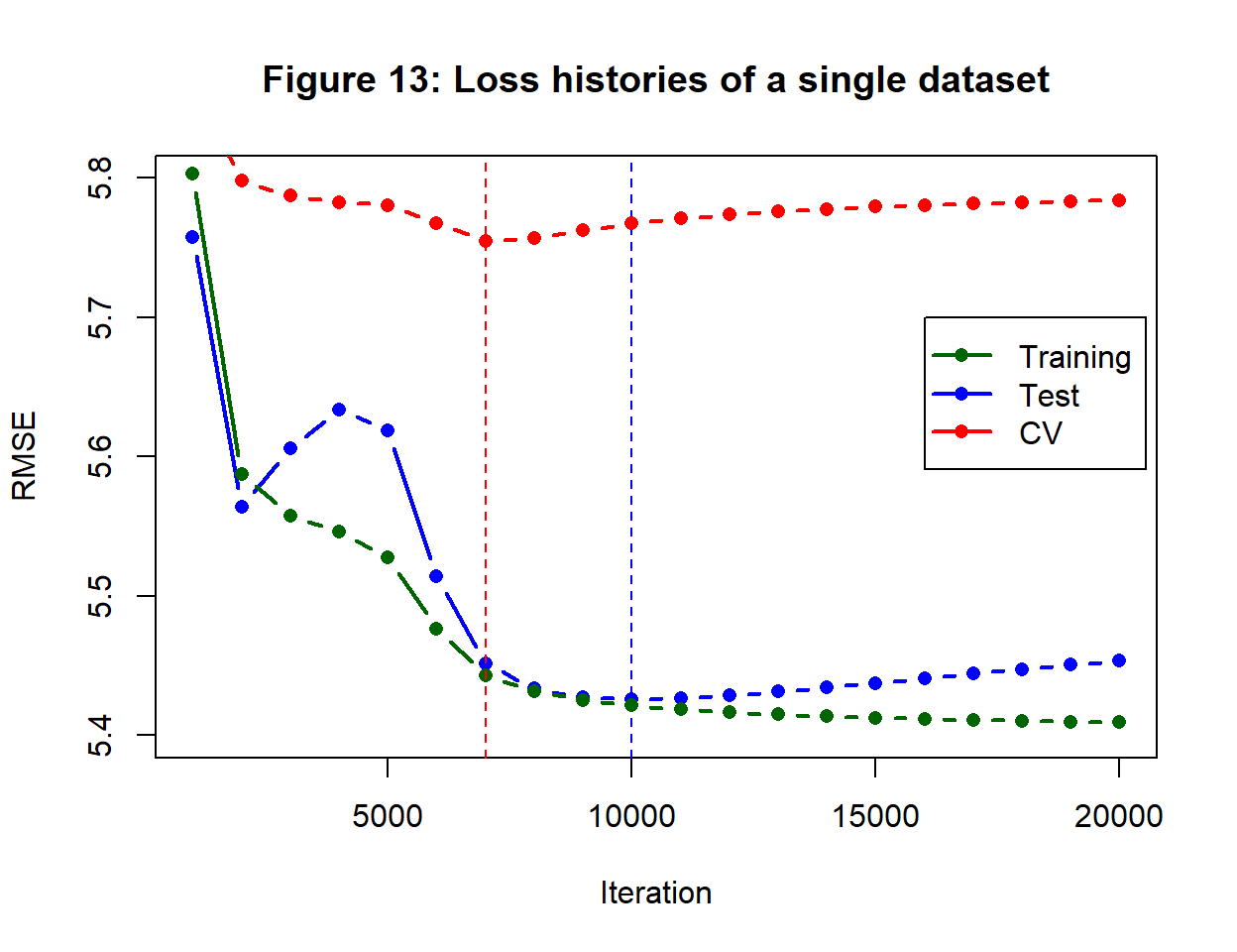
Here are the main points that I take from figure 13.
- training loss decreases steadily throughout, while test and CV loss decrease and then increase
- the change in test loss is erratic early on
- the test loss is lowest when the algorithm is run for 10,000 iterations
- the CV loss is lowest when the algorithm is run for 7,000 iterations
- test loss is the key statistic if you want to choose the best model, CV loss estimates \(L_F\) and is relevant if you want an algorithm that will work well on other sets of training data
- change in CV loss is smooth because the same split was used throughout
- CV loss is much higher that test loss for this particular split. A different split would have produced a red line almost parallel to the one shown, but at a different level.
Although we should not pay too much attention to the level of the CV loss, can we rely on the hyperparameter choice of 7,000 iterations? Figure 14 shows the CV algorithm choice against the test loss algorithm choice for each of the 50 datasets. Larger points mean multiple training sets gave the same pair of losses and results of 20,000 mean that the loss was still reducing when I stopped the search.
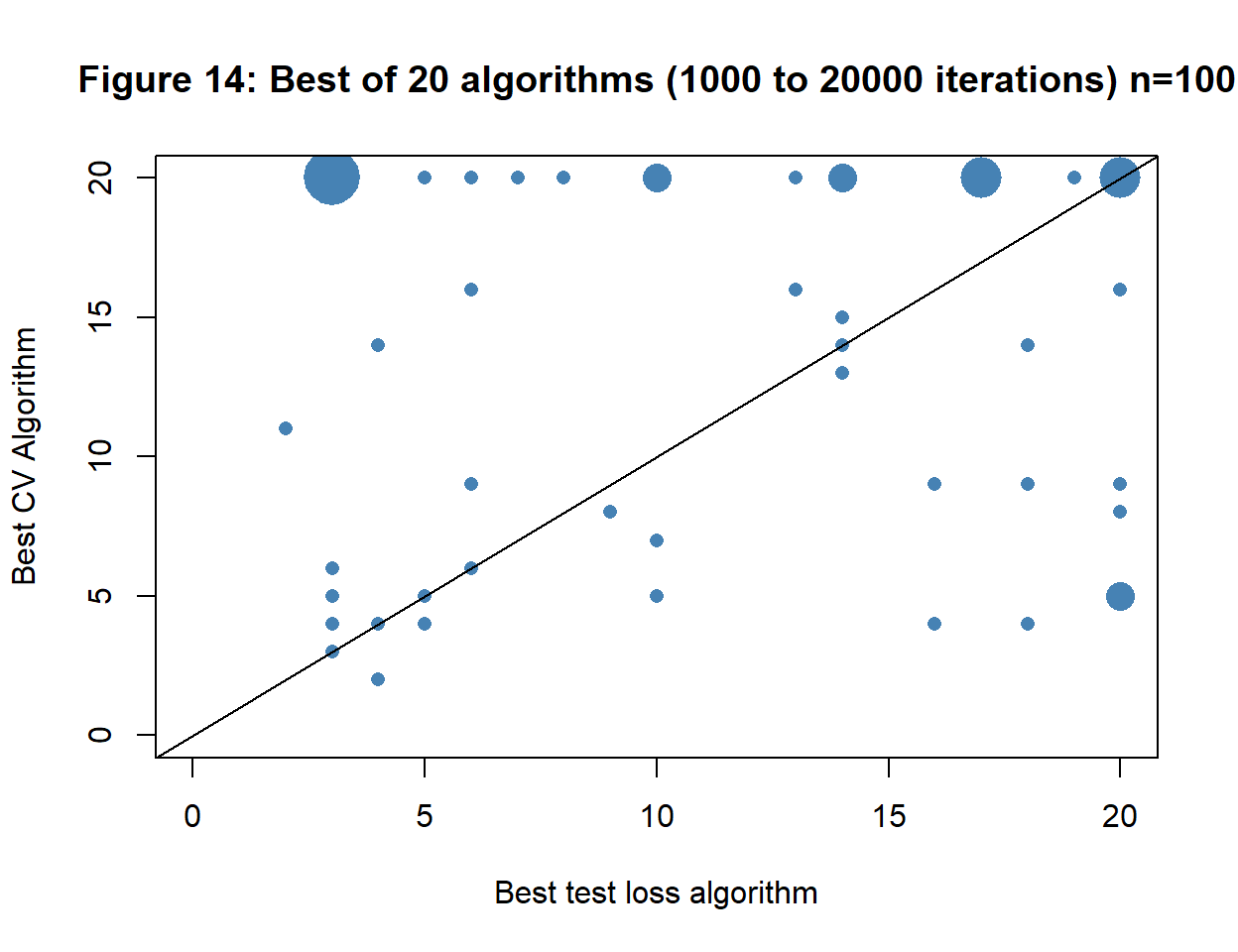
There is little agreement between algorithm choice based on test loss and CV loss. The test loss was still declining at iteration 20,000 in only 16% of the training sets, while the CV loss was still declining in 40%. The median position of the minimum test losses was 10,000 iterations, while the median position for CV loss was 14,000 iterations. The poor performance should not come as a surprise. The sample size is small, as are the performance differences between algorithms a few thousand iterations apart.
Part of the noise in figure 14 is due to the small sample size, so I repeated the analysis with n=400. The algorithms generally need more iterations, so I ran them in steps of 1,000 between 5,000 iterations and 30,000 iterations. The results are shown in figure 15.
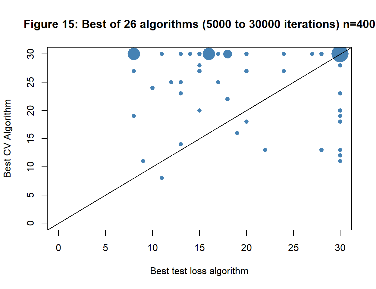
The larger sample size has had little effect on the interpretation, even though the numbers of iterations are slightly higher. There is still little agreement between test and CV loss as to which algorithm is better for a particular dataset. The average choice is slightly higher for CV with a median number of iterations based on CV loss of 23,000 compared with the median of 14,000 iterations for test loss.
If you want to use CV to identify the optimum number of iterations to within a few thousands, then you will need a far larger sample size. Cross-validation with a training set of size 400 would probably distinguish reliably between 10,000 iterations and 50,000 iterations, but would have little hope of reliably distinguishing between 10,000 and 15,000. Without some idea of the resolution of CV it is dangerous to use it.
Conclusions
My interpretation of these simulations is that CV is an imprecise measure of the average performance of an algorithm (\(L_F\)) that provides a poor basis for model comparison and therefore a poor basis for tuning hyperparameters to a particular set of training data, unless the algorithms that you want to compare perform very differently.
Although CV is widely used, I seriously doubt whether close decisions (fine tuning) based on CV have much scientific validity. Many choices made in machine learning are between options that make very little difference to the final outcome in which case using CV does little harm, other than wasting a lot of computer time.
CV provides a high variance estimate of \(L_F\), so it is certainly a mistake to rely on cross-validation for predicting test loss. Having said that, provided that the same split is used for every cross-validation, changes in CV loss are more reliable indicators of relative performance than a single CV is of absolute performance. Differences in CV loss may be ballpark OK for choosing between widely differing algorithms, but they will not be a sound basis for making fine choices. How do you know when two algorithms are far enough apart for CV to distinguish between them? You need an estimate of the standard error of the difference in CV loss, a quantity that is rarely, if ever, mentioned in a report of hyperparameter tuning.
If you plan to use CV for refining an algorithm, you should always estimate the standard error of the difference in CV loss, perhaps by using the bootstrap. This will tell you whether cross-validation has a hope of distinguishing between two algorithms. It only makes any sense to use CV if you are interested in differences in CV loss that are more than, say, 3 times that standard error, otherwise don’t waste your time with cross-validation
There are some alternatives to CV for hyperparameter tuning that are worth considering.
- if the training set is large enough, divide it into holdout validation and test sets plus a smaller training set. Tune the hyperparameters based on the validation loss and predict performance based on the test loss
- base the hyperparameter tuning on external data or prior knowledge (package defaults are based on prior experience and are usually sensible)
- don’t make a choice, but instead average your predictions over models generated by algorithms with different hyperparameters
- use more than 10 bootstrap samples, so that the variance of the loss estimate is smaller than that of 10-fold CV. The bootstrap also uses resampling and has many of the same problems as CV, so don’t take the results too seriously
I cannot say whether these conclusions would remain valid for huge training samples (huge relative to the dimension of the data and number of model parameters); I have not simulated that situation. I suspect that a large training set would reduce the variances, but leave the patterns of behaviour seen in this post unchanged.