Neural Networks: First steps towards a workflow
Introduction
In this series of posts, I am trying to develop a workflow for using neural networks in data analysis. So far, I have developed R code for fitting a neural network (NN) by gradient descent, used Rcpp to convert that code to C for increased speed, pictured the search paths and used NNs to simulate datasets for comparing algorithms. Now I want to start defining the workflow.
Neural networks are flexible models that are usually over-parameterised and as a consequence the surfaces created by their loss functions have many symmetries and multiple local minima. Searching these complex surfaces by gradient descent is slow and computationally intensive making it important that the algorithm is tuned to give it the best chance of finding a good solution within a reasonable time-frame.
Six aspects of the algorithm that must be specified by the data analyst at the outset are,
- the architecture
- the type of activation function
- the scaling of the predictors and responses
- the starting values for the weights and biases
- the step length (learning rate)
- the stopping rule
The first two choices define the model rather than the algorithm and I will leave those choices for another post. The one aspect of the model choice that I will discuss is the centring of the activation function as this affects the efficiency of the algorithm, but leaves the model essentially unchanged.
The other four choices in the list affect the fitting algorithm rather than the model and are inter-related. Rescaling the data affects both the choice of starting values and the choice of the learning rate. When making these choices, we need to balance the desire to find a good model with the computational burden. Running the gradient descent algorithm from 20 different sets of starting values would obviously be better than starting it from 3 different sets, but the gain is unlikely to be worth the effort.
In this post, I will discuss the algorithmic choices in the context of using a NN as a flexible regression model. The post is presented as an investigation; not everything that I tried worked as well as I had hoped, but I think that the failures are themselves quite informative, so I have left them in.
In this post, I cover a lot of ground in a rather superficial way, but at least it is a first step towards developing a general workflow. There is much, much more that can be said about each of these choices, but you have to start somewhere.
Are we talking hyperparameters?
I came to machine learning after a long career in academic statistics, so I bring with me a lot of baggage. In particular, I draw a distinction between a model, such as logistic regression and a fitting algorithm, such as iteratively reweighted least squares. For me, when the model is hierarchical, the higher level model parameters are referred to as hyperparameters. In machine learning, hyperparameters are (usually) tunable features of the algorithm.
There is, in my opinion, a degree of vagueness in machine learning whereby people talk of improvements to the algorithm as if they were improvements to the model. Complaining about this blurring might seem like nit-picking, but it has consequences. For instance, in my next post, I will ask whether cross-validation (CV) measures the performance of the algorithm or the performance of the model? If you use CV, you need to know which it is.
Centring the activation function
The question that I address here is not whether to use one activation function or another. That choice relates to the family of models that is allowed. Rather, I ask how the chosen activation function should be parameterised in order to make the algorithm as efficient as possible.
A NN creates non-linearity and hence its flexibility through its activation function. The popular sigmoid activation function will demonstrate how this works.
The sigmoid
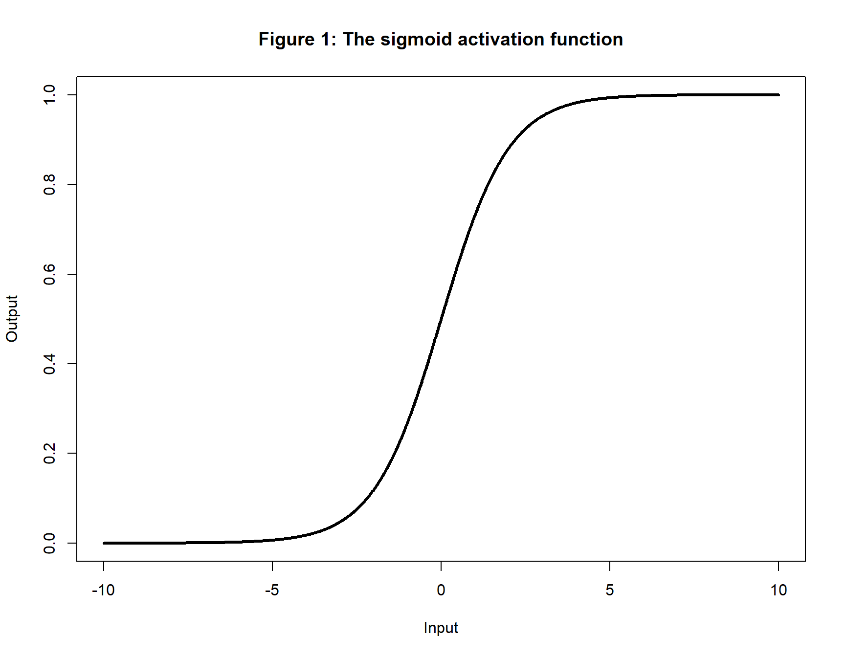
The sigmoid takes the form
\[
y = \frac{1}{1 + exp(-x)}
\]
and its shape is shown in figure 1. The output rises from 0 to 1 as the input goes from about -5 to +5, outside that range the curve is quite flat and almost horizontal.
Suppose that the input to the activation function depends only on a single predictor, x, that varies in size between -1 and 1 and further that the weight of x is 2 and the bias is 1. The input to the activation function will be, z = 1 + 2x and it will take values between -1 and 3. Figure 2 shows the gentle non-linearity that is created under these circumstances. The size of the output is less important than the shape, because the output will be passed on and modified by its own weights and biases.
x <- seq(-1, 1, 0.01)
bias <- 1
weight <- 2
y <- 1 / (1 + exp(-(bias + weight*x)))
plot(x, y, type="l", lwd=3, ylim=c(0,1),
     main = "Figure 2: Sigmoid activation when weight=2 and bias=1",
     xlab="x", ylab="Output")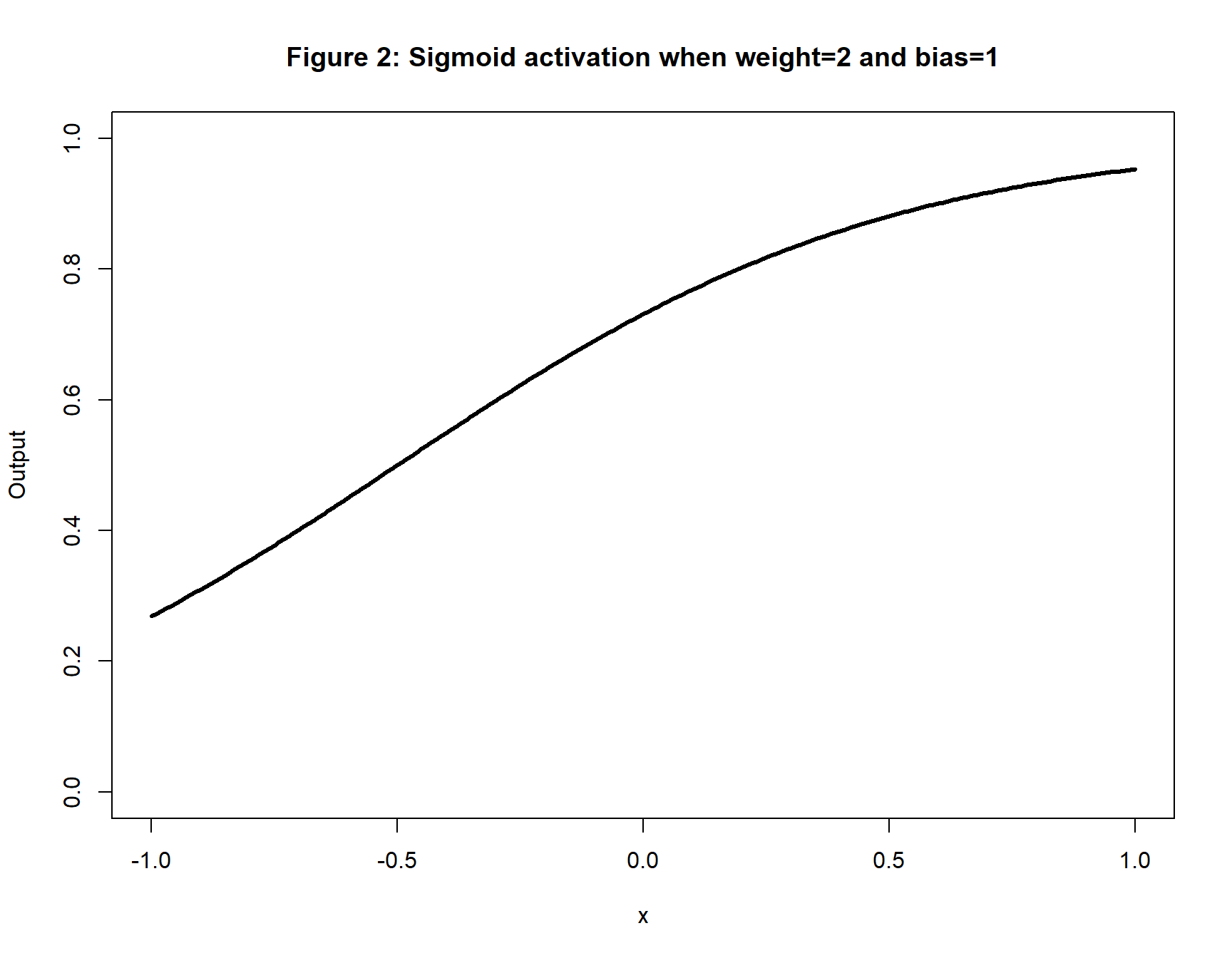
Zero-centred activation
One of the reasons that the tanh function is sometimes preferred to the sigmoid function is that its output range is (-1,1) with a centre at zero, while the sigmoid range is (0,1) with a centre at 0.5. The lack of a zero centre can, of course, be compensated for by adjusting the bias, but doing so creates a correlation between the change that the algorithm makes to the weights and the change needed by the corresponding bias. Gradient descent by back-propagation treats the parameters separately and so does not allow for such a correlation. A large correlation between parameters would cause the gradient descent algorithm to converge more slowly. There is a direct analogy here with the benefits of centring in Bayesian algorithms based on Gibbs sampling.
An alternative to switching to tanh is to keep the sigmoid but to subtract 0.5 from the output so that it is zero-centred and its range is (-0.5, 0.5). The zero-centred sigmoid takes the form, \[ y = \frac{1}{1+exp(-z)} - 0.5 \] and has a derivative given by \[ (0.5 - y)(0.5 + y) \]
Scaling the training data
Were we to use inappropriate weights and biases, it would be easy to force all inputs to the sigmoid activation function to be outside of the range (-5, 5) and hence to make the outputs almost flat and uninformative. The message is that a neural network that uses the sigmoid activation function needs weights and biases that keep most of the inputs in the range (-5, 5). At the same time, the range of values taken by the input must not become too small, or once again the output will not change.
NNs are easier to fit when the predictors in the input layer are all on similar scales and when that scale matches the outcome of the activation function. That way, weights and biases throughout the network will be applied to quantities of a similar magnitude. What we want to avoid is the situation in a weight in one part of the network is say, 1e-5 and a weight elsewhere is 1e9. This would lead to derivatives of greatly varying size and a numerically unstable algorithm. It would also make it difficult to select a step length/learning rate that is suitable for the whole network.
Since the zero-centred sigmoid has an output range of (-0.5, 0.5), it would make sense to scale the predictors in the same way. The exact range is not critical; anything close to (-0.5, 0.5) would do. A simple transformation that would work for well-behaved data is
\[ \frac{x - \text{mid-point}(x)}{ \text{range}(x)} \]
Unfortunately, this transformation would not be very robust. Remember that we are creating an automatic algorithm, so we do not want to inspect each predictor to ensure that there are no outliers distorting the range. Instead, we might use
\[ \frac{x - (\text{Q}_{95}(x) + \text{Q}_{05}(x)) / 2}{ \text{Q}_{95}(x) - \text{Q}_{05}(x)} \]
where \(Q_{05}\) is the 5% quantile. The range of the transformed predictor will be slightly greater than (-0.5, 0.5), but the vast majority of values will be within the target range.
It is common, at least in regression problems, not to apply an activation function to the final output of the network, that way the output can take whatever value is appropriate to the response of the particular problem. To help make all weights and biases have a similar order of magnitude, the final outputs to the network will need to be scaled so that they too have a value in the range (-5, 5). A possible robust transformation is,
\[ \frac{10 \ (y - (\text{Q}_{95}(x) + \text{Q}_{05}(x)) / 2)}{\text{Q}_{95}(y) - \text{Q}_{05}(y) } \]
Starting Values
The requirement that inputs to a zero-centred sigmoid activation function are in (-5, 5) while the outputs are in (-0.5, 0.5), suggests the use of weights in the range (-10, 10). However, when there are many inputs to a node, the weight given to each one needs to be reduced. Suppose that a particular node has L inputs, we might expect the weights to be in the range (10/L, 10/L). In fact, this is a little conservative because there may be some cancellation with some of the inputs being positive when others are negative. A sensible compromise is, \[ \left( \frac{-10}{\sqrt{L}} , \frac{10}{\sqrt{L}}\right) \]
This type of weight adjustment has been suggested many times based on more mathematical derivations, for example, He et al ( arXiv:1502.01852) suggested that the weights should be reduced by the square root of L for the ReLU activation function and Glorot and Bengio (“Understanding the difficulty of training deep feedforward neural networks.” International conference on artificial intelligence and statistics. 2010) suggested reducing by the root of the number of inputs plus the number of outputs.
The biases are added to the weighted combination of the inputs and the final result needs to be in (-5, 5), so certainly most biases will need to be within this range.
Neural networks are full of symmetries, for instance we could swap any two nodes in a layer provided that we also swap their input and output parameters. By having a good variety of starting weights and biases, you increase the chance of hitting on something close to one of the symmetrical minima. The general rule is that convergence will be quicker when the starting values are not all similar.
Step length (Learning rate)
I am torn between referring to the step length, as one would in statistics, and the learning rate, as one would in machine learning. In the context of gradient descent they mean the same thing, but step length is a little more descriptive, so I will go with that.
Choosing the step length is not trivial, but there are some intuitions that might help guide us
- too small a step length and progress towards the minimum will be slow
- too large a step length and the algorithm might jump over the minimum leading to oscillation or even divergence
- it makes sense to start with a large step length and to decrease it as we approach the minimum
- a good step length for one parameter might not be ideal for other parameters, although scaling the data will greatly reduce this problem
- the more parameters in the model the smaller the step length, because each iteration changes all of the parameters simultaneously
- a small step length will enable the exploration of small features in the surface of the training loss. However, such narrow features are likely to be specific to the particular training dataset and so might not generalise. Broad minima are more important because they reflect trend rather than noise.
Common-sense intuitions are useful, but they are not evidence, and we need to keep in mind that there will be times when even the best intuitions fail us.
Constant step length
Finding a good step length is often a matter of trial and error. Typical values lie between 0.0001 and 1.0, so a sensible strategy would be to try a range of values, perhaps 0.0001, 0.001, 0.01, 0.1 and 1.0 and run each for a small number of iterations to see what happens. Select the largest step length that does not cause oscillation or divergence.
Scheduled step length reduction
Instead of picking a value, the step length could be allowed to start high and decrease slowly. A schedule that I like is to divide the iterations into 20 equal sized blocks, then each time the algorithm moves to a new block, the size of the step length is reduced by 10%. 0.9^19=0.13 so the size of the step length in the final block will be about 13% of the size of the original; start with 0.1 and you will end with something close to 0.01.
Automatically adjusted step length
Instead of deciding in advance on the schedule of step lengths, adjustment could be made to depend on the progress of the algorithm. As the algorithm approaches the minimum, it will occasionally over-shoot, causing the loss to oscillate or diverge. At that point, the step length should be reduced.
A simple rule is; if the training loss increases, reduce the step length and use parameter values somewhere between the previous values and the new values.
Should you decide not to use automatic adjustment, it is still important to monitor for oscillation and/or divergence, either by visual inspection of the output of the algorithm, or by detecting an increase in the loss and flagging it. This information might make you re-run the analysis, or at the very least, it will inform future analyses.
Stopping Rules
With neural networks, the gradient descent algorithm tends to progress through cycles with periods of rapid improvement followed by longer periods when progress almost plateaus. You do not want to stop the algorithm during a plateau, if a period of rapid improvement is still to be reached. At the same time, the algorithm cannot be allowed to go on forever in the vain hope of improvement.
The stopping rule could be based on changes to the training loss, or to changes to the parameters, or to the sizes of the derivatives. When automatic step length adjustment is used, it is important that a minimum step length is specified, so that the algorithm does not make countless negligible changes.
So far the discussion has assumed that the goal is to stop when the algorithm reaches a minimum in the training loss. As I explained in my post on search paths, the real aim is to minimise the expected loss and not the training loss. I will consider early stopping based on expected loss in my next post, which is on cross-validation.
Another limit of this investigation is that I assume that the neural network is not so over-parameterised that the loss can be reduced to zero. Such models can exhibit strange behaviour, such as a test loss that increases and then comes down again. Another topic for a future post.
Possible strategies
In my investigation, I planned to use simulated data to compare two strategies
Option A
- unscaled data
- standard sigmoid activation
- starting weights and biases that are random Uniform(-1, 1)
- fixed step length of 0.1
- 10,000 iterations
Option B (my preference)
- robust scaling of predictors to approximately (-0.5, 0.5)
- robust scaling of responses to approximately (-5, 5)
- zero-centred sigmoid activation
- starting biases random Uniform(-5, 5)
- starting weights random Uniform(-10/sqrt(L), 10/sqrt(L))
- automatically adjusted step lengths starting with 0.1
- stop when percentage change in the training loss drops below 1e-3, or at 10,000 iterations whichever comes sooner
Option A was a straw man set up to fail, but unfortunately I overdid it. Without scaling, gradient descent gets stuck and, even in my very simple examples, one million iterations still got nowhere near the solution. To make a practical comparison, I need to introduce some scaling of X and Y.
The eventual comparison that I ran was between option B and a modified version of option A.
Option A
- scale the predictors and responses by subtracting their mean and dividing by their standard deviation
- standard sigmoid activation
- starting weights and biases random Uniform(-1, 1)
- fixed step length of 0.1
- 10,000 iterations
Comparison 1: The Wave
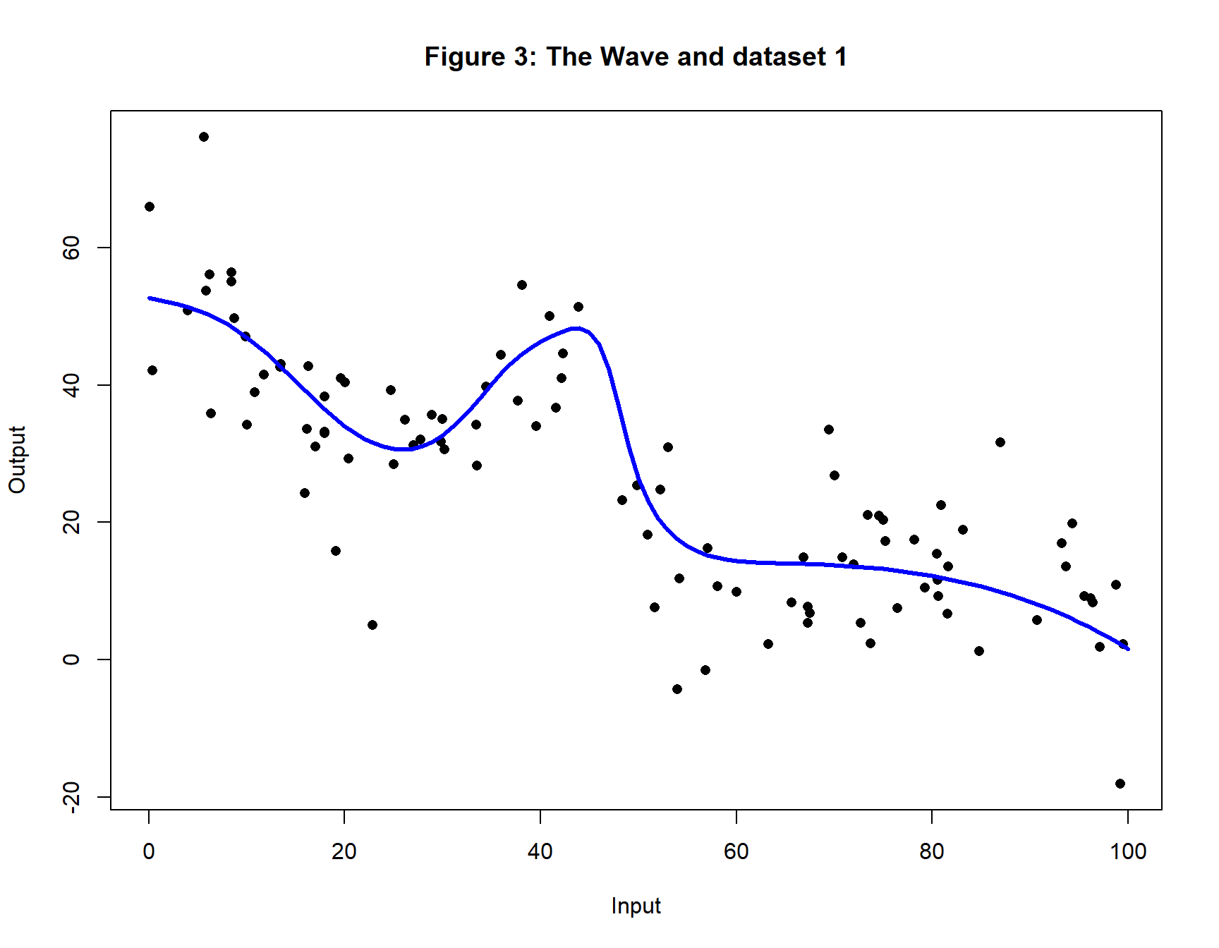
My first comparison is based on a simple regression. Using the method described in my previous post, I used a (1, 4, 8, 4, 1) NN with different randomly generated weights and biases and a standard sigmoid activation function to create a simulated dataset. Figure 3 shows the relationship between the input and the output and a single set of 100 training values. I call it a wave to make it easier to refer to.
The model
The simulated data are analysed using a (1, 8, 1) NN. The model is fitted to 20 randomly generated sets of training data from the wave. Each dataset is analysed three times from different starting values. All of the analyses are performed once with Options A and once with B. A test set of 10,000 observations was used to estimate the expected loss. The training and test RMSE were recorded over 10,000 iterations (sometimes called Epochs). The randomness in the simulation was such that true curve has an expected RMSE of 8.
All calculations were run using the Rcpp code for gradient descent as described in previous posts. The code is available on my GitHub pages at https://github.com/thompson575/NeuralNetworks. I make a few adjustments to the code to accommodate the stopping rules and step length adjustments. These changes are described in an appendix at the end of this post.
An example of fitting the model
Figure 4 illustrates the performance of Option A. The blue curve is the wave used in the data generation. The other lines show progress of the NN fit after 1,000 iterations (dashed orange), 2,000 iterations (dashed pink), 5,000 iterations (dashed light green) and 10,000 iterations (solid dark green).
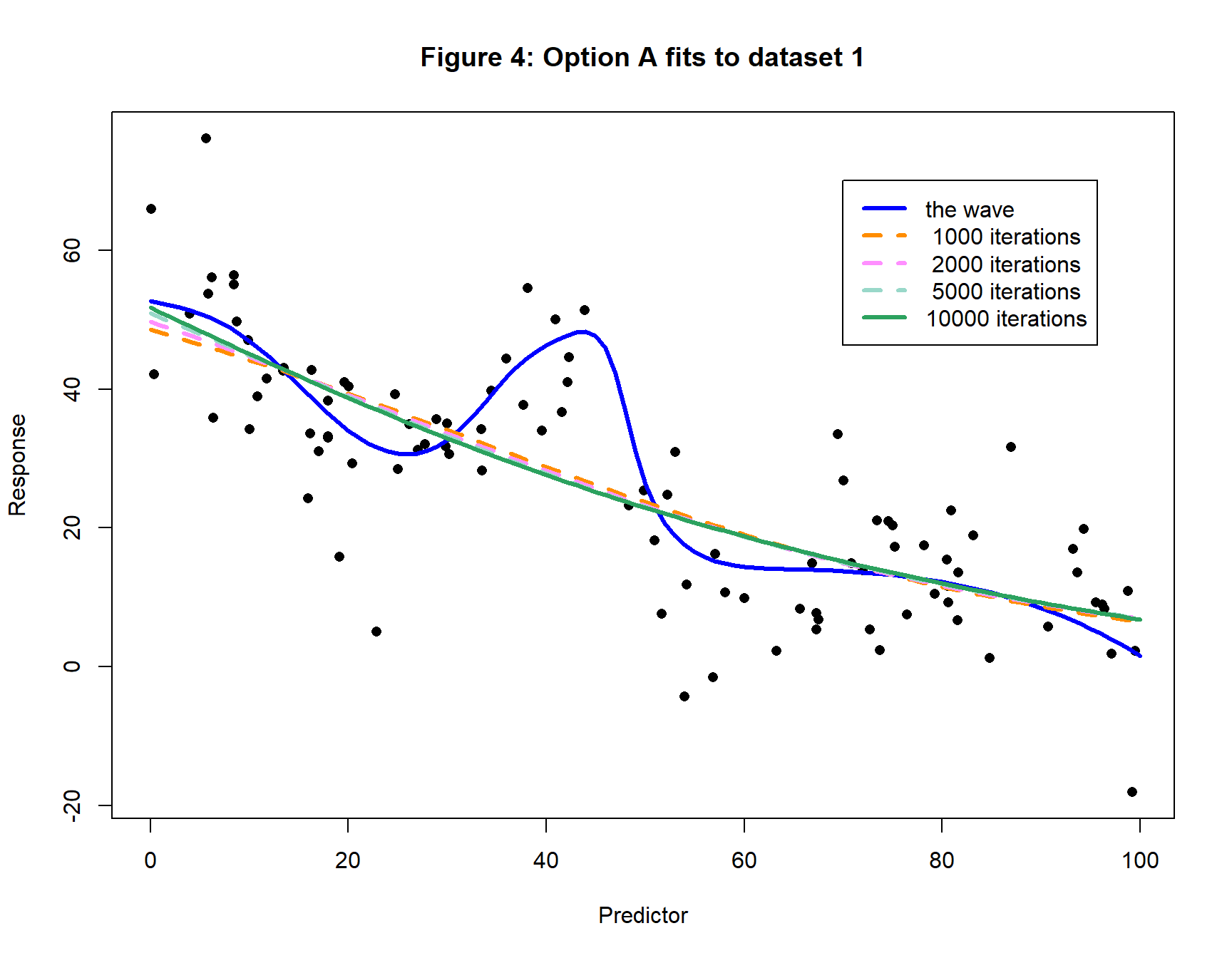
This example shows that quite early on Option A fits a straightish line and then makes little progress over the 10,000 iterations.
Figure 5 shows the corresponding plot to figure 4 for Option B. The algorithm makes progress, but has not yet matched the wave.
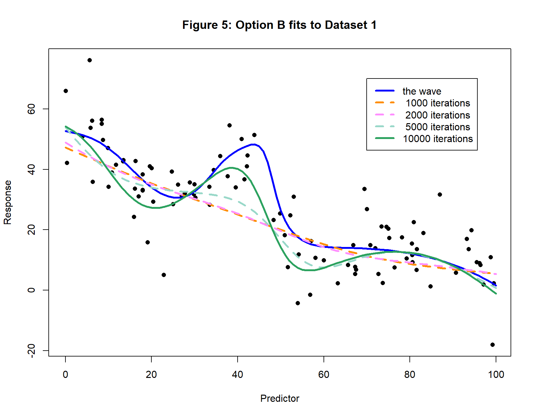
The full set of results for each of the 20 datasets is shown in table 1. For each curve the tabulated value refers to the replicate (from the three sets of starting values) that achieved the final lowest test loss.
The benefit from using Option B is clear.
| Table 3: Wave Datasets | ||||||||
| Best Test RMSE per dataset by Iterations | ||||||||
| iterations | ||||||||
|---|---|---|---|---|---|---|---|---|
| dataset | Option A | Option B | ||||||
| 1,000 | 2,000 | 5,000 | 10,000 | 1,000 | 2,000 | 5,000 | stop | |
| 1 | 10.70 | 10.80 | 10.80 | 10.80 | 10.50 | 10.30 | 9.58 | 8.72 |
| 2 | 10.60 | 10.50 | 10.30 | 9.94 | 9.89 | 9.28 | 8.30 | 8.26 |
| 3 | 10.30 | 10.10 | 9.71 | 8.43 | 9.89 | 9.29 | 8.26 | 8.20 |
| 4 | 10.40 | 10.40 | 9.61 | 8.41 | 10.40 | 10.30 | 8.85 | 8.29 |
| 5 | 10.40 | 10.40 | 10.20 | 9.62 | 9.97 | 9.70 | 8.61 | 8.18 |
| 6 | 10.70 | 10.70 | 10.70 | 10.80 | 10.50 | 10.20 | 9.72 | 8.40 |
| 7 | 10.60 | 10.70 | 10.30 | 9.21 | 10.50 | 10.40 | 9.65 | 8.60 |
| 8 | 10.40 | 10.30 | 10.00 | 9.05 | 10.00 | 9.82 | 8.87 | 8.15 |
| 9 | 10.30 | 10.20 | 10.10 | 9.85 | 10.10 | 9.89 | 9.03 | 8.40 |
| 10 | 10.30 | 10.20 | 9.90 | 8.31 | 10.30 | 10.10 | 9.77 | 8.28 |
| 11 | 10.40 | 10.40 | 10.20 | 9.88 | 10.30 | 10.20 | 9.55 | 8.72 |
| 12 | 10.30 | 10.20 | 9.95 | 9.75 | 10.20 | 10.10 | 9.25 | 8.12 |
| 13 | 10.30 | 10.20 | 9.94 | 9.72 | 9.64 | 8.84 | 8.23 | 8.19 |
| 14 | 10.40 | 10.30 | 9.98 | 8.48 | 10.10 | 9.76 | 8.40 | 8.26 |
| 15 | 10.70 | 10.60 | 10.30 | 9.55 | 10.50 | 10.30 | 9.61 | 8.64 |
| 16 | 10.40 | 10.40 | 10.30 | 10.10 | 10.30 | 10.20 | 9.00 | 8.26 |
| 17 | 10.40 | 10.30 | 10.10 | 9.34 | 10.10 | 9.97 | 8.35 | 8.08 |
| 18 | 10.60 | 10.50 | 9.47 | 8.33 | 10.30 | 9.47 | 8.34 | 8.33 |
| 19 | 10.60 | 10.60 | 10.60 | 10.40 | 10.20 | 9.95 | 8.90 | 8.60 |
| 20 | 10.60 | 10.60 | 10.60 | 10.50 | 10.30 | 10.10 | 8.71 | 8.39 |
Option A only obtained a test loss below 9 by iteration 10,000 in 5 of the 20 datasets. Option B finished close to 8 in every case and never ended with a higher test loss than option A.
To see if Option A would eventually find a good solution, the analysis for dataset 1 was run for 100,000 iterations. As I am interested in computational efficiency, figure 6 plots the training and test losses against iteration number. The analysis was repeated three times with different starting values, shown in blue, red and green. The blue and red curves happen to be very similar.
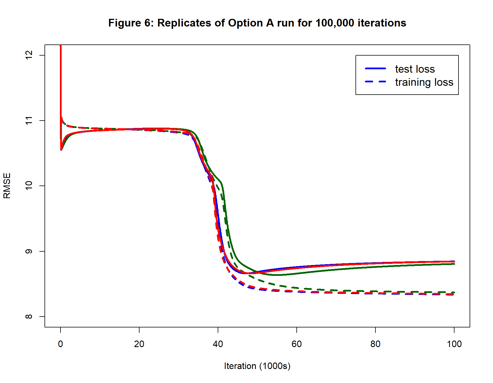
10,000 iterations was clearly far too few. Each of the sets of starting values found their fitted model after around 50,000 iterations. The minimum test RMSE was 8.66, slightly lower that the solution obtained by Option B, but Option B stopped at 9,014 iterations due to my stopping rule.
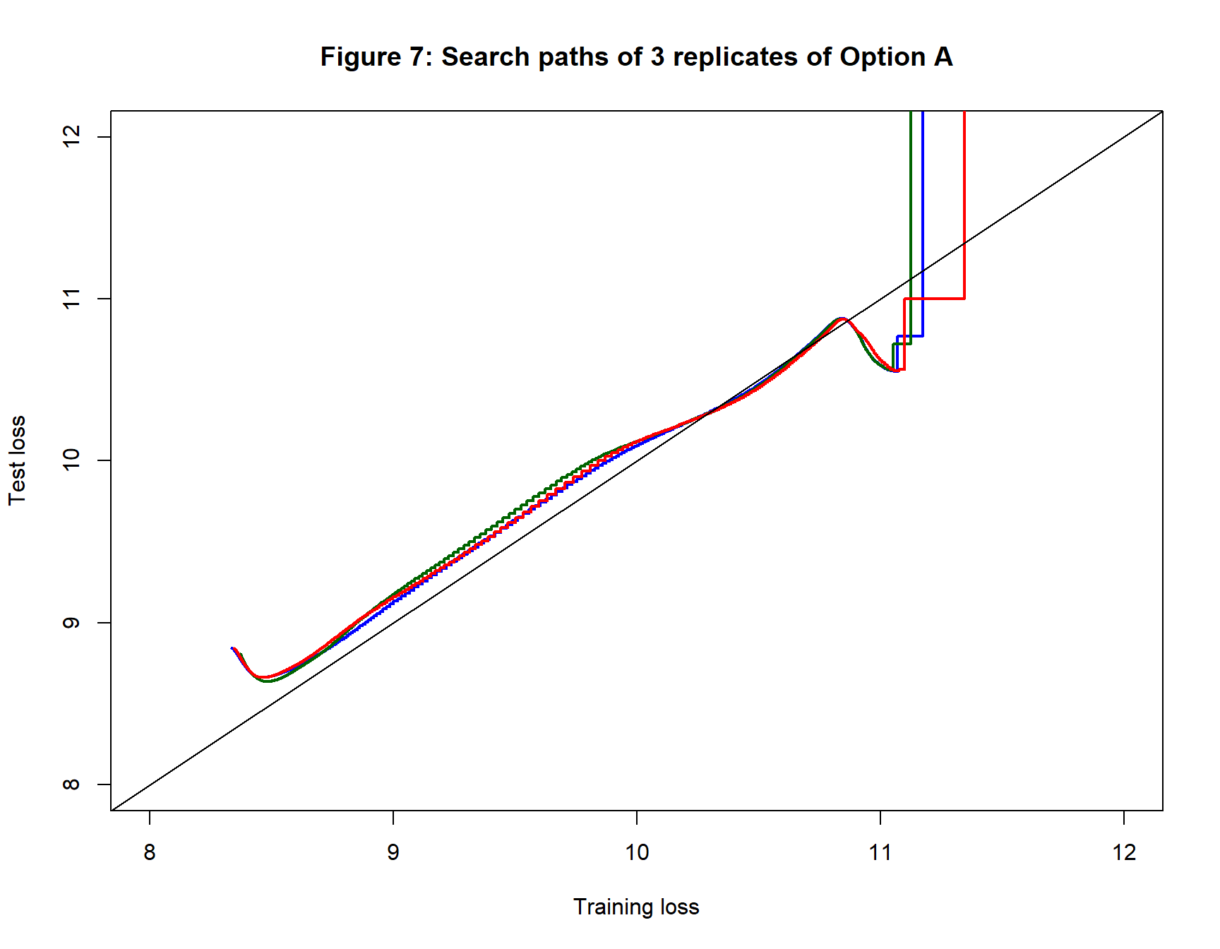
Figure 7 shows the search paths. The curves appear as steps because, to save time, the test loss was only calculated every 50 iterations. The three sets of starting values produce very similar search paths.
My conclusions from this example are
- Option B is preferable to Option A
- Option A gets there in the end, but is inefficient
- My choice of stopping rule stopped Option B too soon
- It is not clear what aspect of Option A caused it to converge so slowly
Reasons the for poor performance of Option A
To investigate where Option A goes wrong, I tried four changes (keeping everything else the same).
- switch to the zero-centred sigmoid
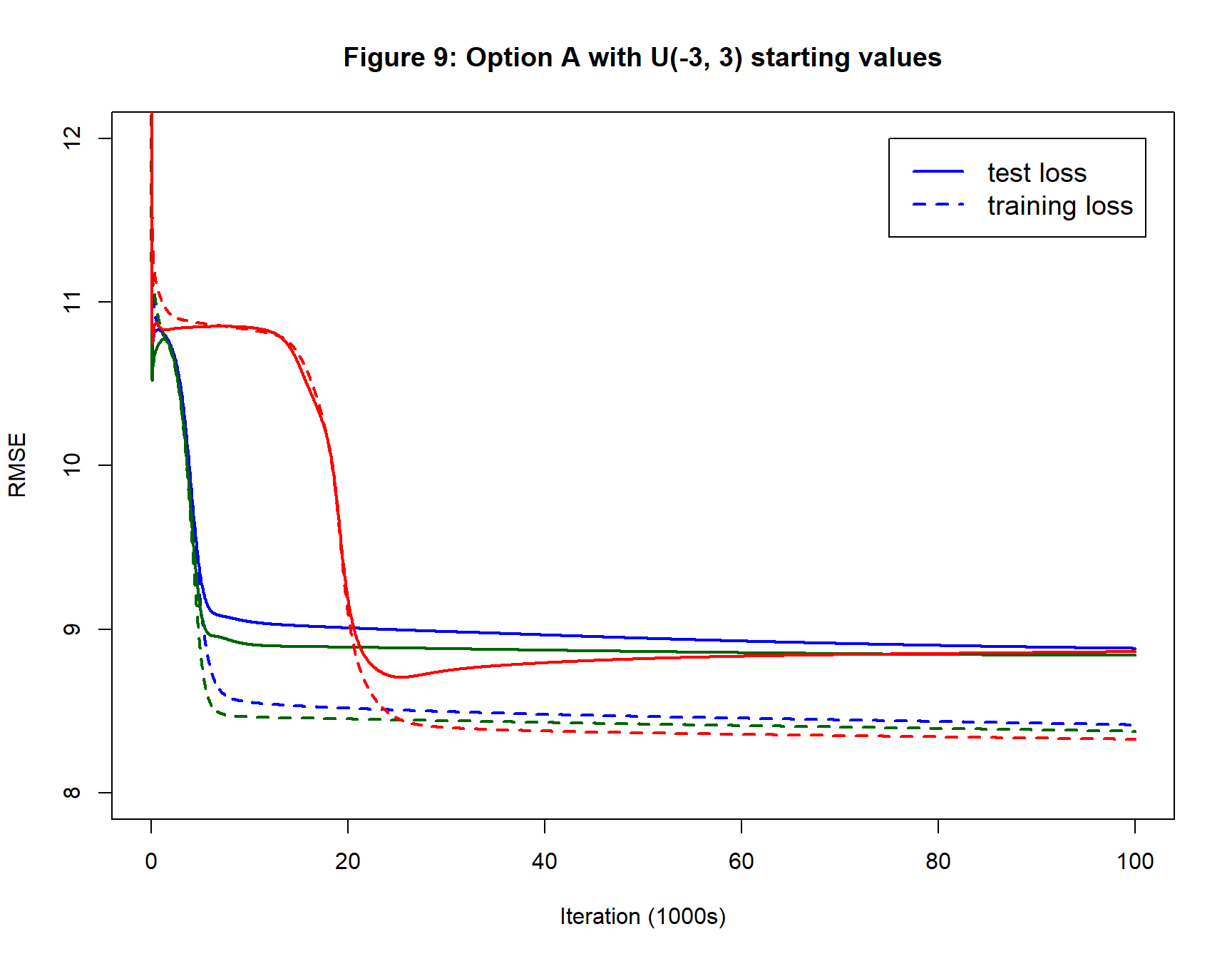
- draw starting values from U(-3, 3) instead of U(-1, 1)
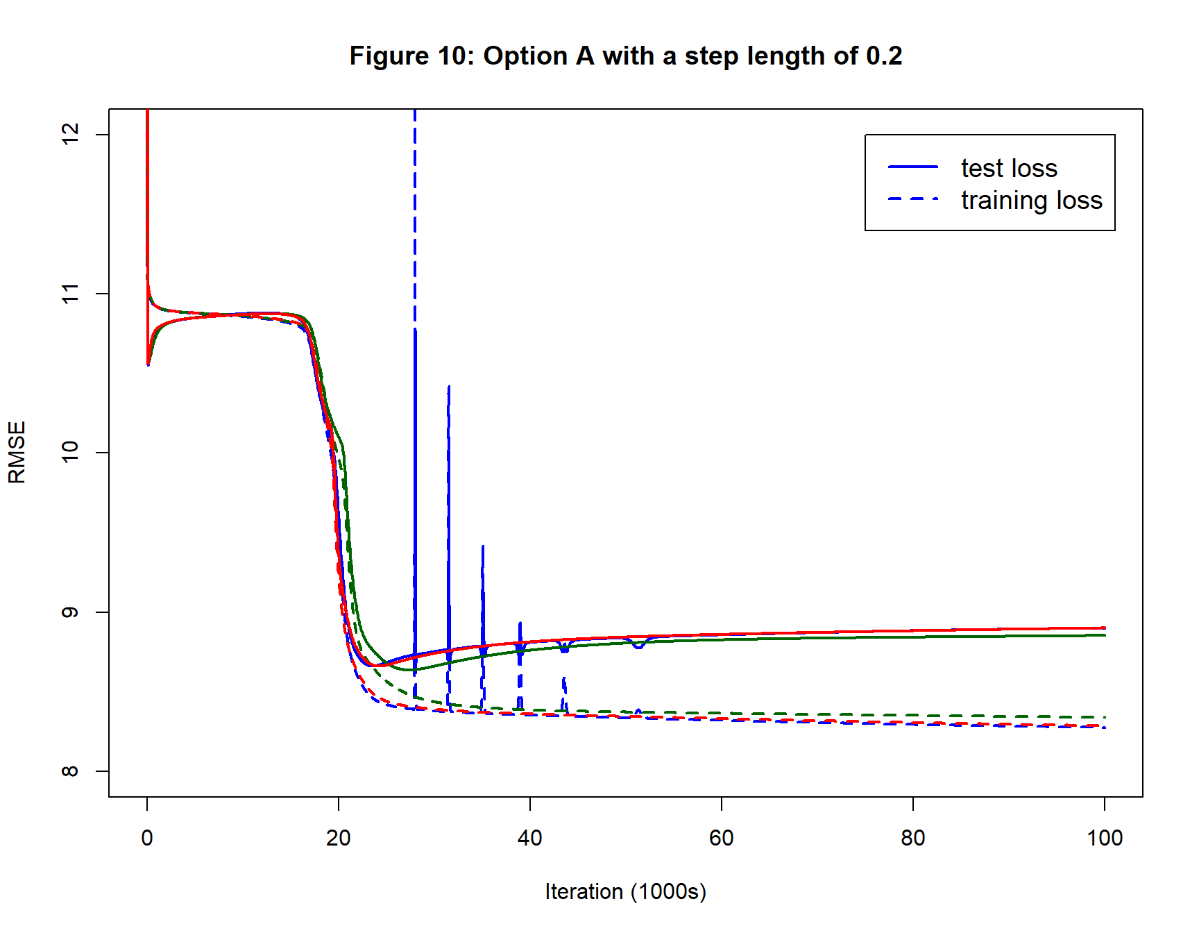
- increase the step length from 0.1 to 0.2
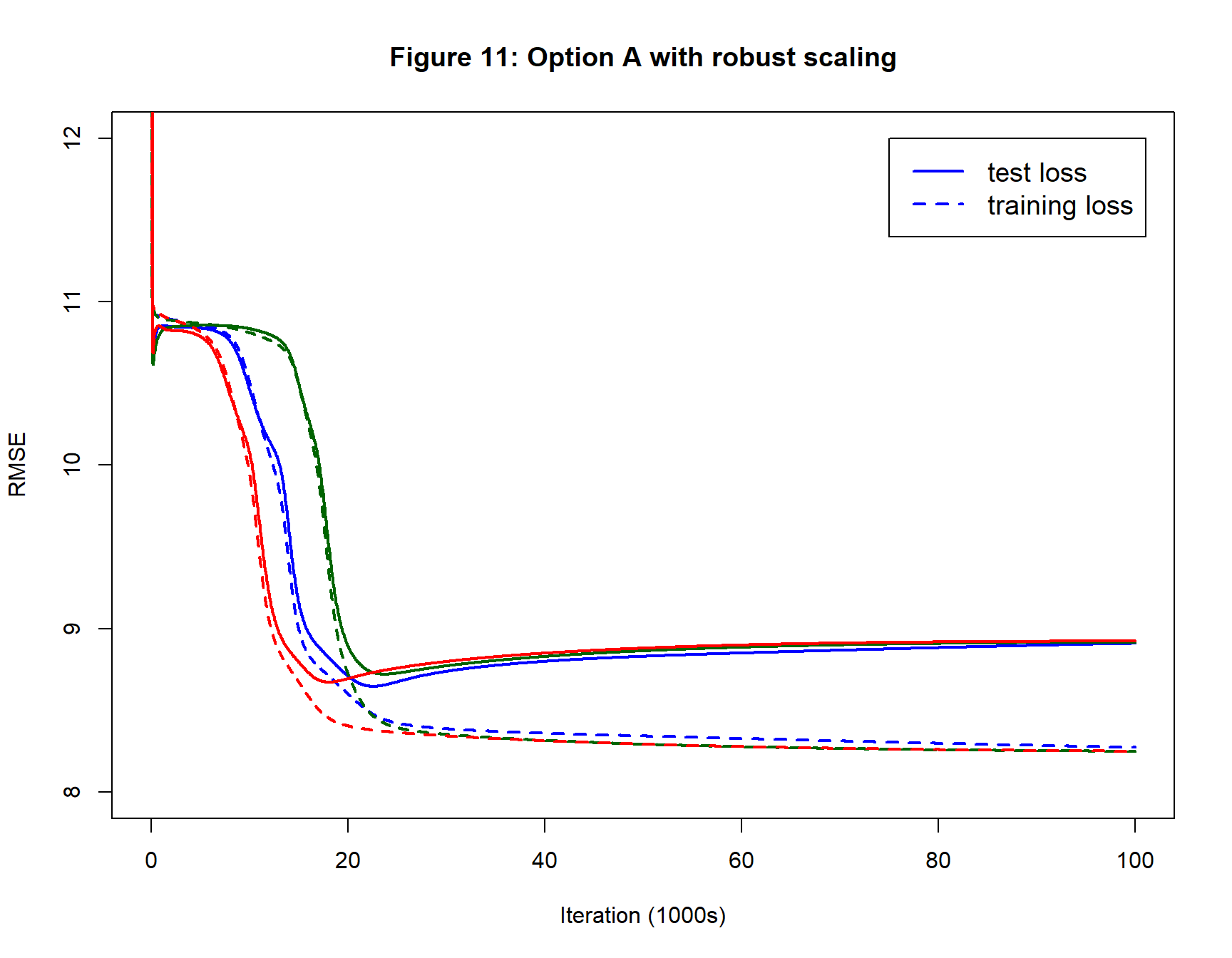
- use robust scaling
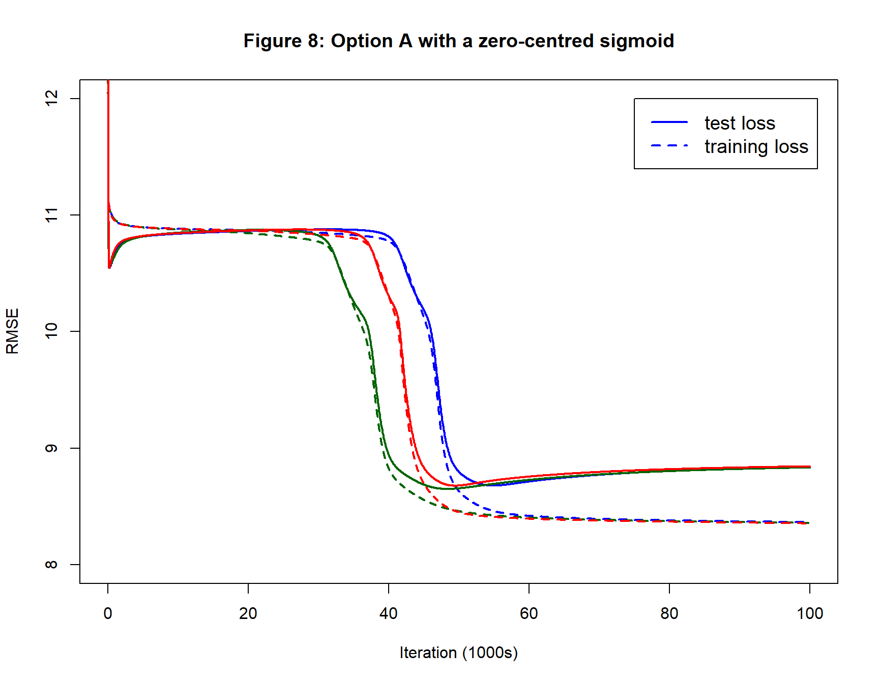
Zero-centred sigmoid
Figure 8 shows that performance is similar to vanilla Option A with the optimum model obtained after 40,000 to 50,000 iterations.
Larger starting values
Figure 9 shows that increasing the range of starting values creates a faster initial improvement but it makes the final performance worse. There is more variation between the replicates and only the red replicate finds a minimum for the test loss. The blue and green test losses are still decreasing after 100,000 iterations.
Larger step length
Figure 10 shows the impact of doubling the step length. The fitted model is now found after around 25,000 iterations rather than 50,000. For the blue replicate the convergence is not smooth, the search regularly over-shoots the loss and has to recover.
Robust Scaling
Figure 11 shows the impact of using robust scaling. Progress is smooth and the minimum test loss is found after about 20,000 iterations. This is by far the best version of Option A, but it is still not as good as Option B.
Final conclusions about Option A
Activation function, scaling, starting values and step length all seem to play a role in determining performance and no doubt they interact, but of the four the scaling of the data seems to be the most important. A larger initial step length speeds convergence, but causes over-shoot, perhaps automatic reduction of step length would help.
Comparison 2
My second comparison is based on a single dataset of n=1000 observations with 6 inputs (predictors, X) and one output (response, Y). The data were generated in such a way that the correct model would have an expected RMSE loss of 1. The training data are shown in figure 12.
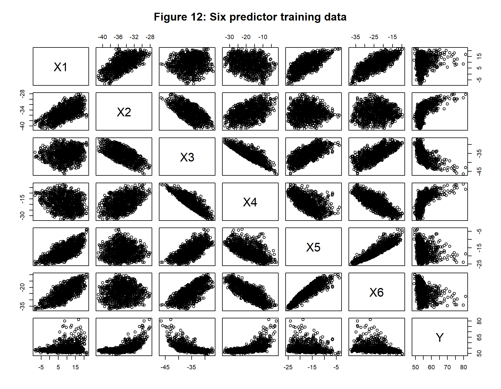
These data are analysed with a (6, 10, 1) neural network. Option A and B are run as originally defined except that I ran 50,000 iterations and a stopping rule for Option B based on a 1e-5 percent change in the loss. Figure 13 shows the patterns of loss by iteration. Option B converges sooner, as we might have anticipated from the first comparison.
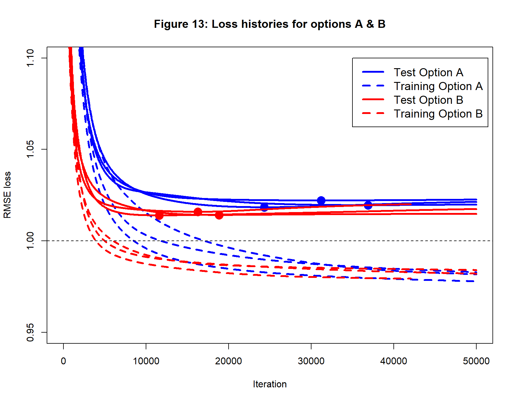
The test loss of the fitted models is quite a bit lower with Option B suggesting that Option A has converged to a slightly worse solution for all three sets of starting values. This can be seen more clearly from the search paths in figure 14.
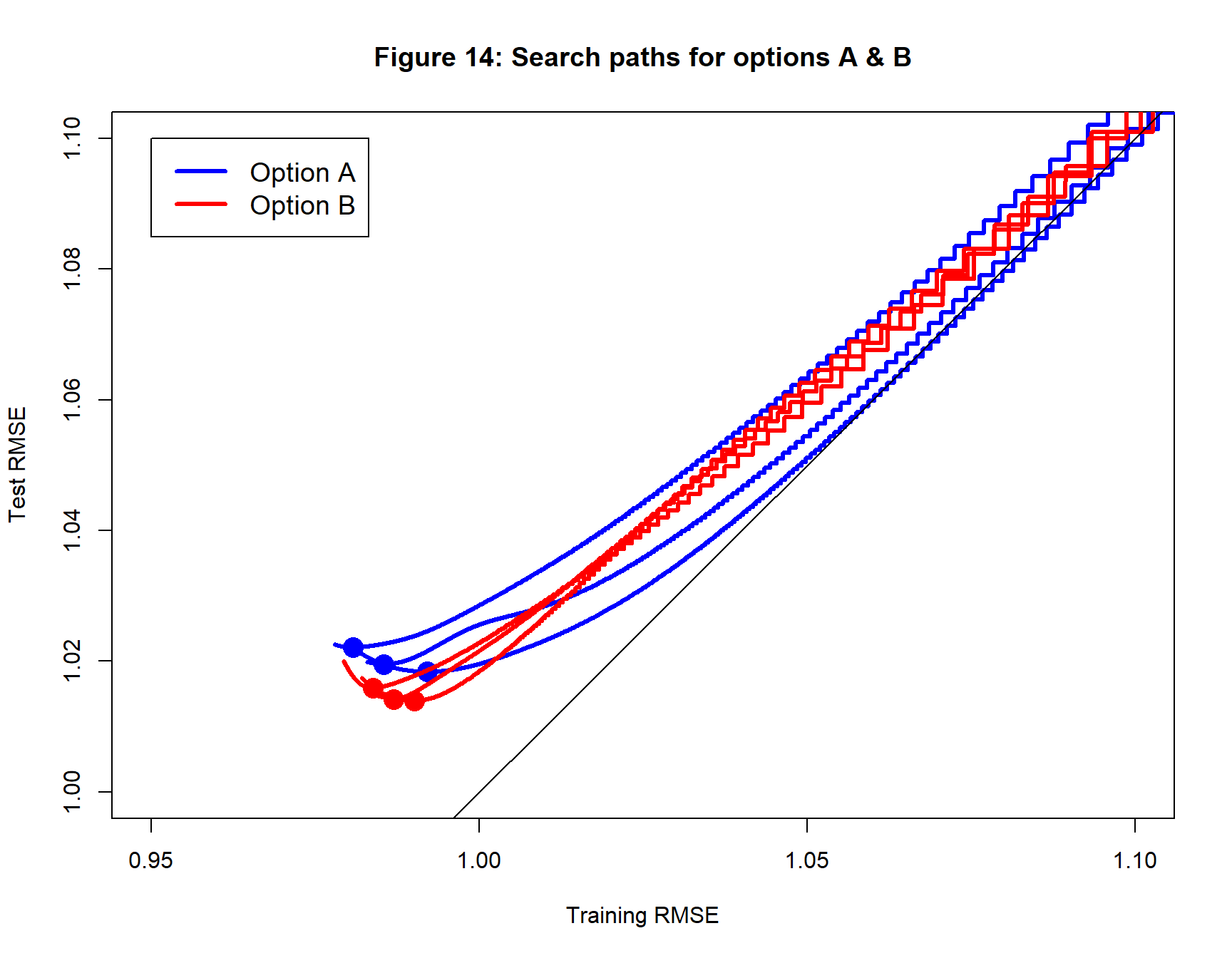
Conclusions from comparison 2
This comparison also strongly favours Option B. Not only is the fitted model found in about half the time, but the test loss of the solution is lower.
Summary
This has been a rather meandering investigation that has raised as many questions as it has answered. Here are the points that I take from it.
- some scaling of the predictors and responses is essential
- starting values need to be ball-park sensible so that inputs stay within the active part of the activation function
- the exact choice of starting values and step length affects the speed of convergence more than the final solution
- models that look very different can actually be equivalent - there are many symmetries in the loss function of a neural network
- Option B performed much better than Option A
I am very aware that these conclusions need to be confirmed in a much greater range of scenarios, but I suspect that Option B would prove to be sensible for a wide range of problems. I will use it in future posts and refine it as necessary.
In practice, the time taken by the gradient descent algorithm means that it is only suitable for small sets of training data; stochastic gradient descent (SGD) works better for larger datasets and so it is not worth putting too much effort into refining the gradient descent workflow, when the real need is for a workflow for SGD.
Appendix: Code Changes
The C code used in this post can be found on my GitHub pages as cnnUpdate02.cpp.
I added options to cfit_nn() and cfit_valid_nn() to give the use the possibility to
- use of the zero-centred sigmoid
- report the loss to a specified schedule
- use scheduled step length reduction
- automatically halve the step length if the loss increases
- calculate the test loss to a specified schedule
- stop early when changes in the training loss are small
The C function Lin() returns the number of inputs to the node served by each weight.