Neural Networks: Data - Real and Simulated
Introduction
In this series of posts, I aim to develop a workflow for using neural networks in data analysis. So far, I have developed R code for fitting a neural network by gradient descent, converted that code into C for increased speed and discussed the workings of the gradient descent algorithm, stressing the importance of the expected loss.
This post considers the data that I will use to test aspects of the neural network (NN) workflow and concentrates mainly on simulation. The methods discussed require a few minor tweaks to my C Code that I describe in a brief appendix.
The advantages of simulation
Simulated data enable experiments in which the true underlying model is known and the expected loss can be calculated. Here are just a few of the things that could be investigated using simulated data.
- aspects of the data
- the impact of the size of the training set
- the impact of the form of the underlying trend
- the impact of the amount of error in the response
- the impact of correlation between the predictors
- the impact of outliers
- the impact of measurement error in the predictors
- the impact of the size of the training set
- aspects of the model fitting algorithm
- the impact of the model architecture
- the impact of the choice of activation function
- the impact of the choice of loss function
- the impact of the starting values
- the impact of regularization
- the impact of the choice of stopping rule
- the impact of the model architecture
My plan is to use these and other investigations to define a workflow for using NNs in a data analysis and then to test the best strategy on real data.
Performance measures
Simulation experiments are usually comparative, for instance, the comparison of a workflow with and without regularization. Such experiments need performance measures that summarise the differences. As I mentioned in my last post, the performance of a specific model is best judged by its expected loss, which can be approximated using a second large dataset that is independent of the training data. One of the big advantages of simulation is that test data of any size can be produced.
When the aim is to identify a method of analysis that is applicable to a wide range of problems, the performance of the fitted models needs to be averaged over a range of scenarios and a range of training datasets.
The most frequently used performance measures are
- the training loss
- the expected loss (approximated using a large test set)
- the cross-validation loss
- the time or number of iterations to convergence
These measures need to be averaged over multiple sets of training data generated from the same underlying model with decisions based on the average performance, although the variance in performance may also be interesting. When one of the simulated datasets produces extreme performance, either good or bad, it is important to discover the causes of the unexpected result, as these might give a clue to ways in which the workflow could be improved.
Sometimes it is informative to calculate performance locally, that is to say over subsets of the training or test data. For example, a NN used for regression, might produce good predictions when the true response is small, but give unreliable predictions when the true response is large.
Neural Networks for Simulation
One of the most difficult design considerations in a simulation study is the choice of the true underlying relationship between the inputs and the outputs. This needs to be complex enough to challenge the model, but not so complex that it is unrealistic. It is often said of simulation studies that whatever method you advocate, you can always find some structure that will show your choice of method in a good light. If you want to develop a good workflow, then it is important to establish that it works well across a wide range of scenarios.
Neural networks (NNs) are designed to create very flexible models, so if you want to simulate data with a wide variety of different relationships, why not use a NN?
Single input, single output
Suppose that we were to take a basic NN, say (1, 10, 1), which is to say, a single predictor X, a single response, Y, and a single hidden layer with 10 nodes. The plots below show Y against X for randomly generated sets of biases and weights and a sigmoid activation function.
# The design
arch <- c(1, 10, 1)
design <- cprepare_nn(arch)

# sequence of values for the predictor
Xs <- matrix(seq(0, 1, 0.02), ncol=1)

# create 9 different sets of weights & biases
par(mfrow=c(3,3))
for( s in 2670:2678) {
  set.seed(s)
  # random parameters
  design$bias   <- runif(length(design$bias), -3, 3)
  design$weight <- runif(length(design$weight), -10, 10)
  # predicted response under the model
  Ys <- cpredict_nn(Xs, design, actFun=c(1, 0))
  # plot of the relationship
  plot(Xs[, 1], Ys[,1], type="l", main=paste("seed=",s), ylab="Y", xlab="X")
}
mtext("Random Curves", side = 3, line = - 1.5, cex=1.5, outer = TRUE)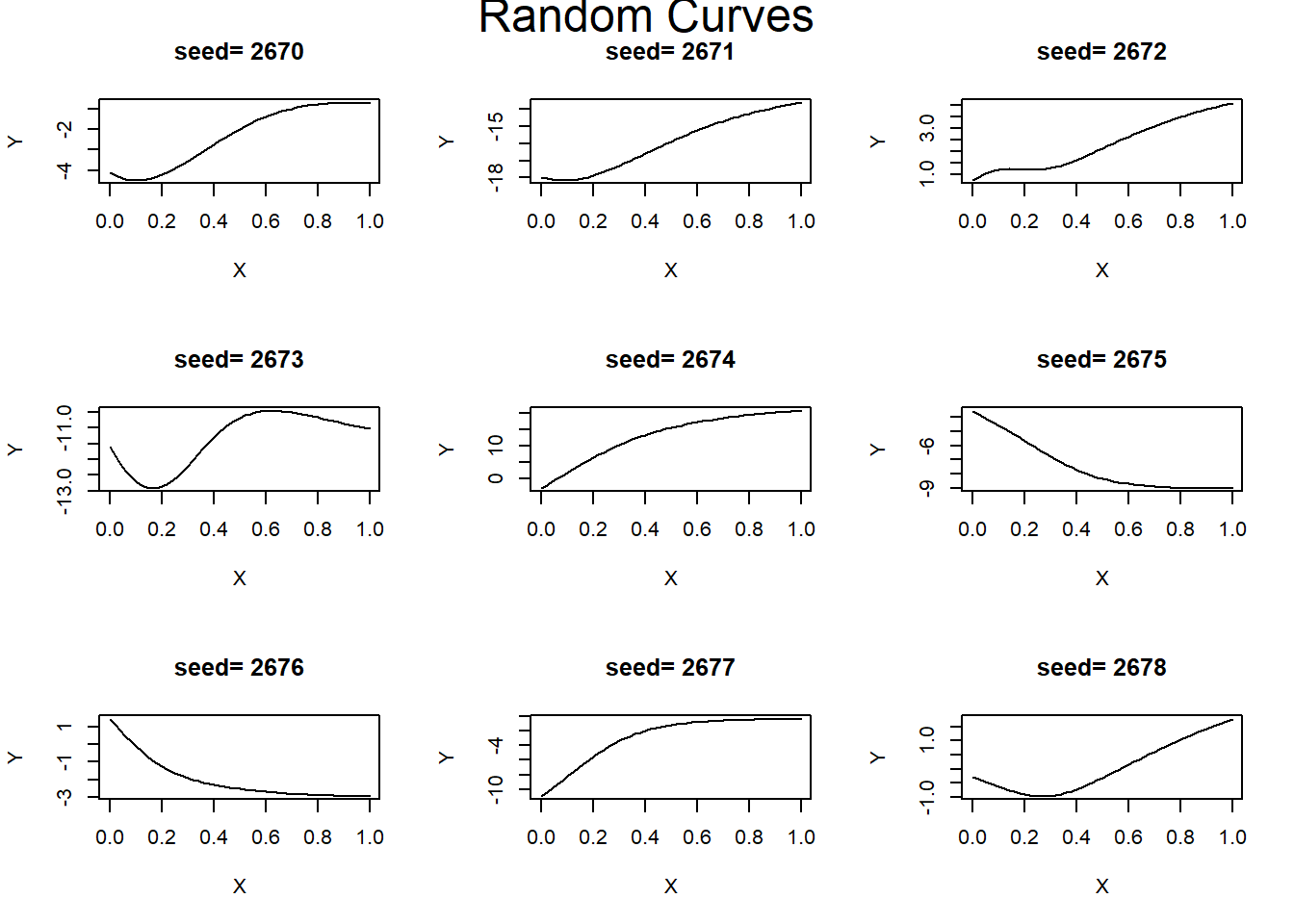
par(mfrow=c(1, 1) )Training data can be generated by adding noise to the response. For clarity of presentation, the datasets plotted below have only 50 observations.
# random values for the predictor
set.seed(4678)
X <- matrix(runif(50, 0, 1), ncol=1)

# create 9 different sets of weights & biases
par(mfrow=c(3,3))
for( s in 2670:2678) {
  set.seed(s)
  # random parameters
  design$bias   <- runif(length(design$bias), -3, 3)
  design$weight <- runif(length(design$weight), -10, 10)
  # predicted response at the plotting points
  Ys <- cpredict_nn(Xs, design, actFun=c(1, 0))
  # predicted response for the random predictors
  Y <- cpredict_nn(X, design, actFun=c(1, 0))
  # add noise to the response
  Y[, 1] <- Y[, 1] + rnorm(50, 0, 1)
  # plot the training data
  plot(X[, 1], Y[,1], main=paste("seed=",s), pch=16, ylab="Y", xlab="X")
  lines(Xs[, 1], Ys[, 1])
}
mtext("Random Data", side = 3, line = - 1.5, cex=1.5, outer = TRUE)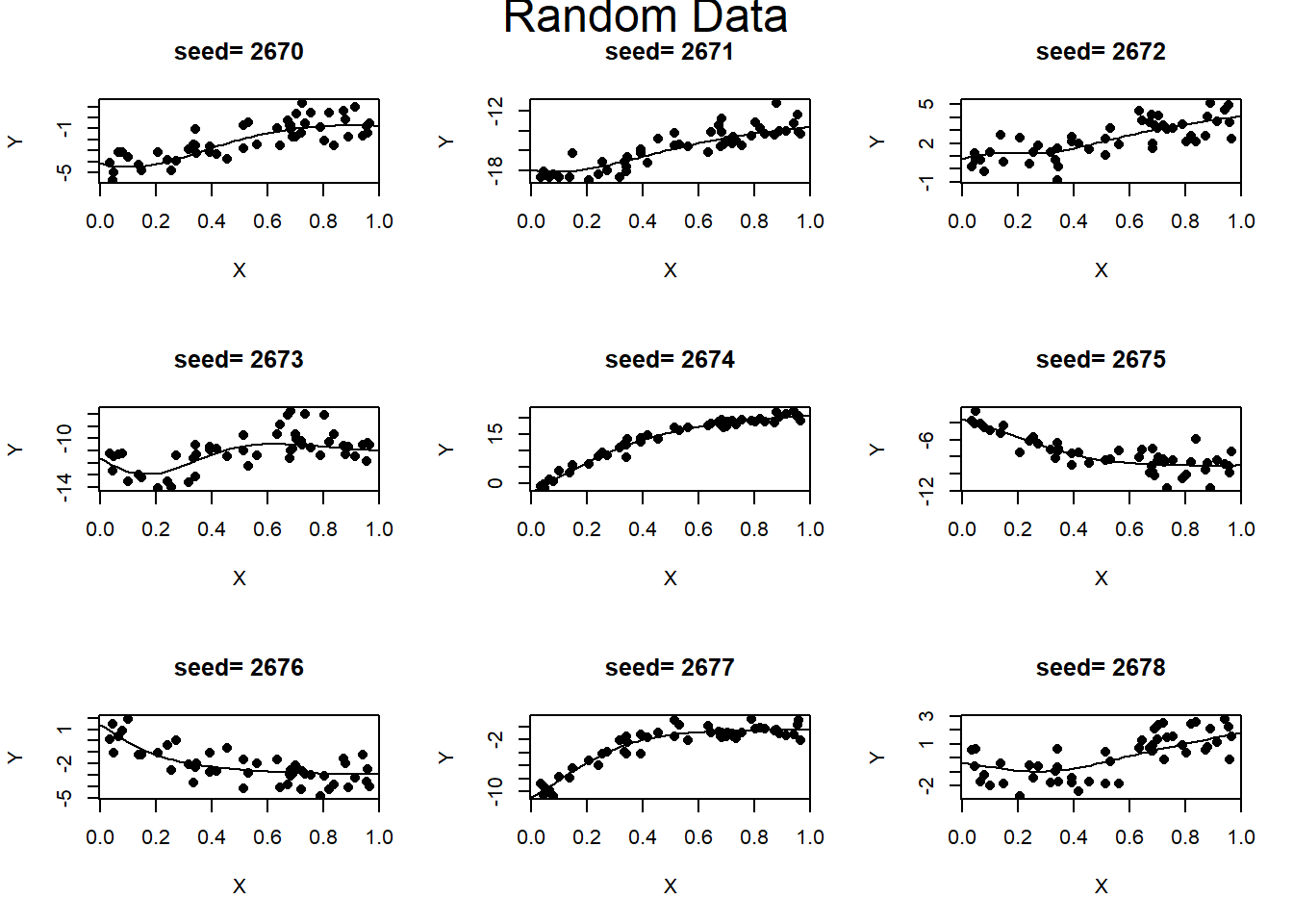
par(mfrow=c(1, 1) )Increasing the size of the noise would obviously make the underlying pattern harder to find.
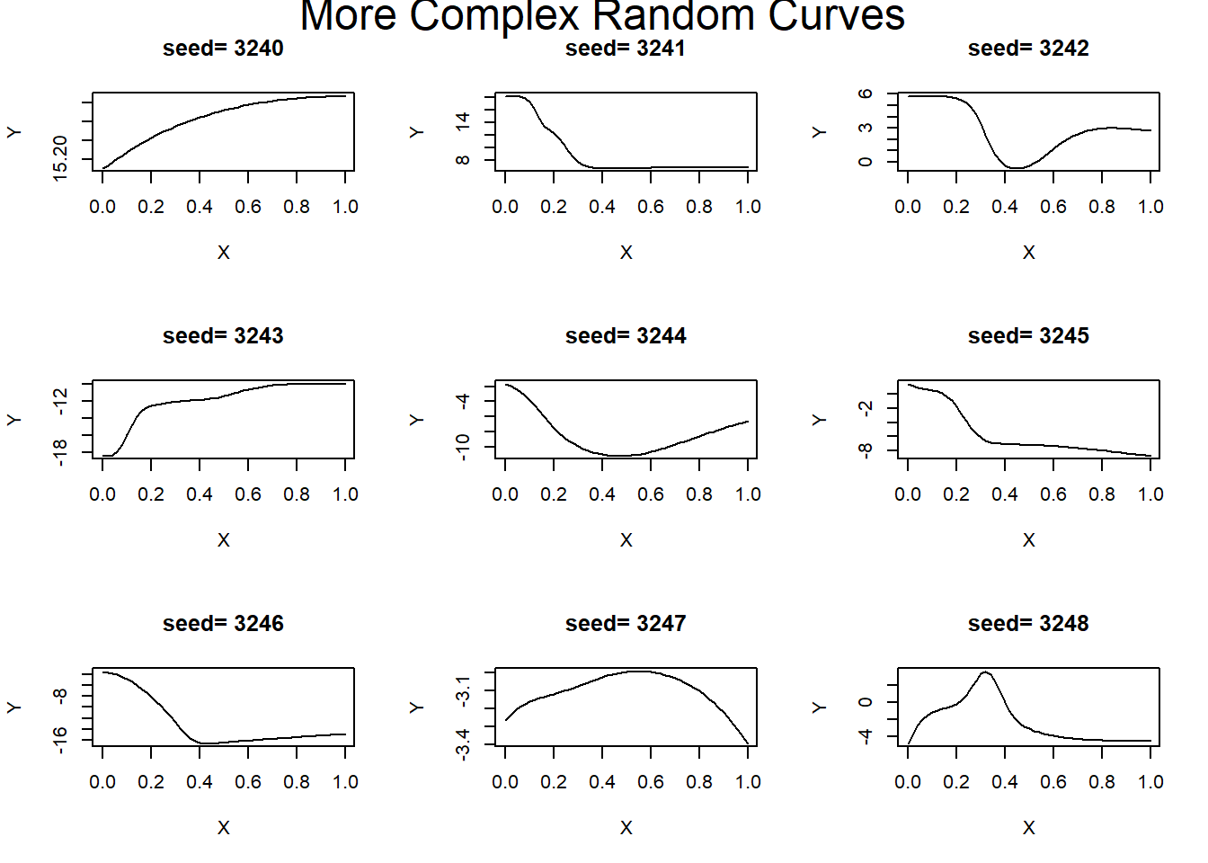
For more complex underlying curves, just use a NN with more parameters. The following examples use random weights and biases in a (1, 8, 8, 1) NN.
Multiple inputs, single output
This method is not restricted to a single input, a (5, 6, 1) NN has 5 inputs and one response.
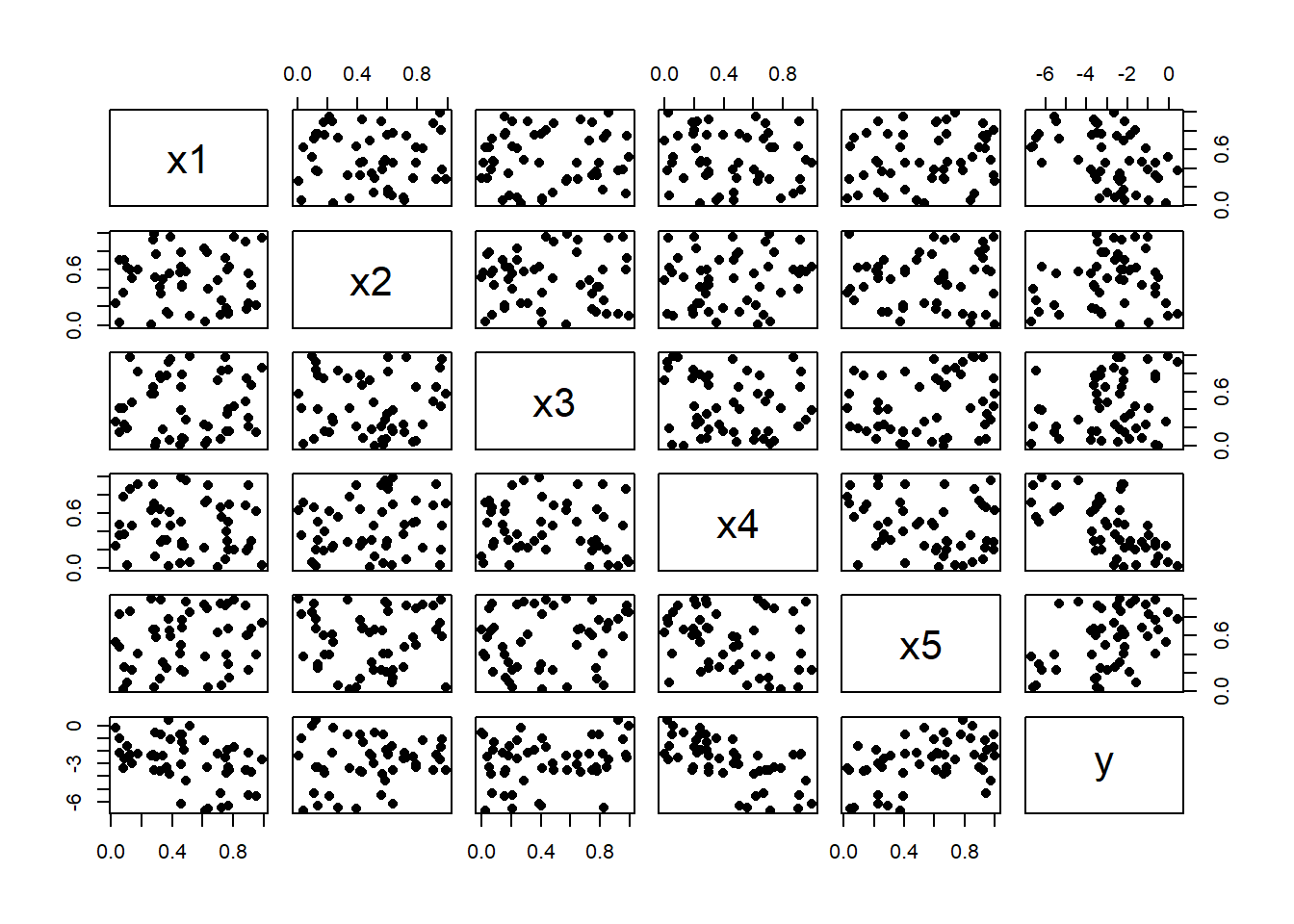
This simulation creates five independent uniform(0, 1) predictors that show no relationships in the plots. There is a relationship between the x’s and the response y and, as no noise has been added, the relationship is a smooth high dimensional response surface, although it is impossible to see that from these marginal plots.
It might be more realistic to have predictors that are not independent, perhaps a (2, 6, 5) NN could be used to create five correlated predictors.
# The design
arch <- c(2, 6, 5)
design <- cprepare_nn(arch)
set.seed(3281)
# random values for the two generators
U <- matrix(runif(100, 0, 1), ncol=2)
# random parameters
design$bias   <- runif(length(design$bias), -3, 3)
design$weight <- runif(length(design$weight), -10, 10)
# create the predictors from the generators
X <- cpredict_nn(U, design, actFun=c(1, 0))
colnames(X) <- paste0("x", 1:5)
# matrix plot of predictors
pairs( X, pch=16)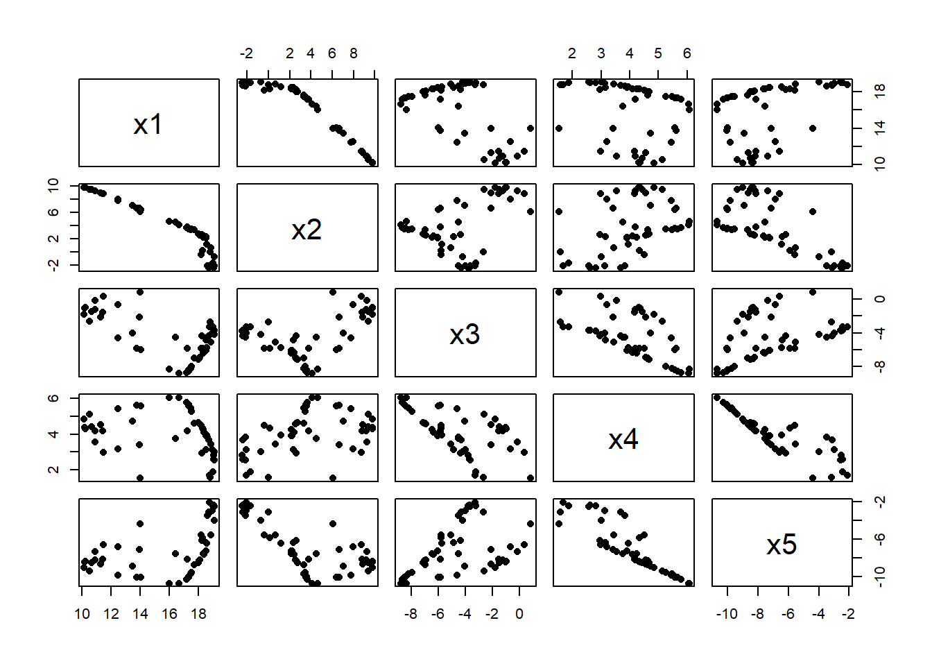
Now a (5, 6, 1) NN adds the response
# The design
arch <- c(5, 6, 1)
design <- cprepare_nn(arch)
set.seed(3281)
# random parameters
design$bias   <- runif(length(design$bias), -3, 3)
design$weight <- runif(length(design$weight), -10, 10)
# response
Y <- cpredict_nn(X, design, actFun=c(1, 0))
colnames(Y) <- "y"
# matrix plot of predictors and response
pairs( cbind(X, Y), pch=16)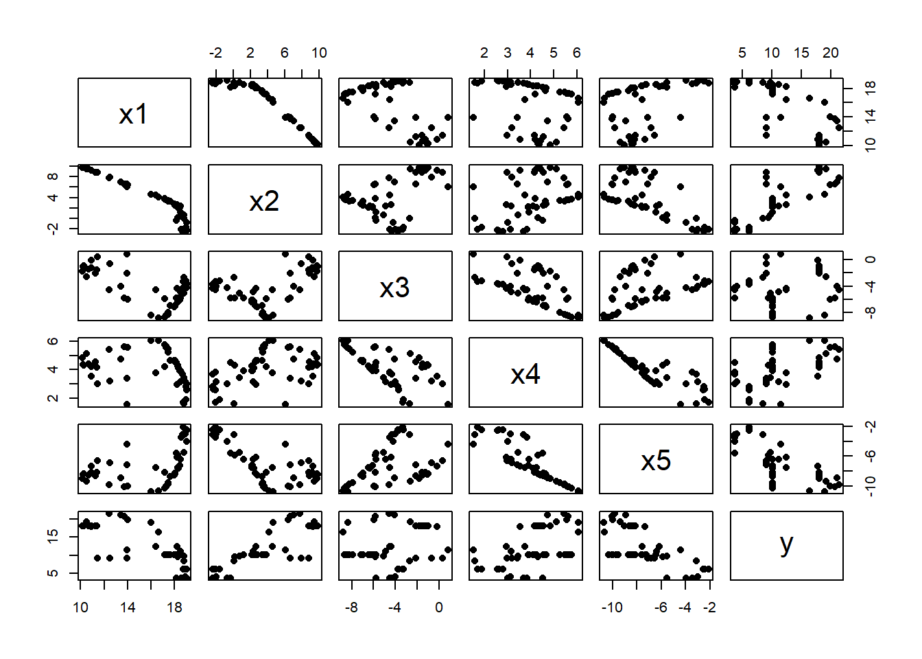
Here is the matrix plot with noise added to the response
# add noise to the response
Y[, 1] <- Y[, 1] + rnorm(50, 0, 1)
# matrix plot of predictors and response
pairs( cbind(X, Y), pch=16)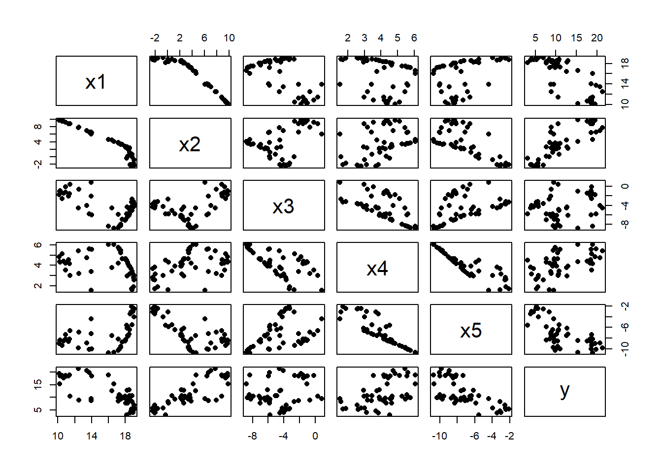
There are strong patterns between the X’s and a more obvious relationship with Y. The more generators, U, that are used when creating the predictors, the weaker will be the associations between the X’s.
I am sure that you are ahead of me in seeing that this simulation could have been created from a single run of a (2, 6, 5, 6, 1) neural network. Layer 3 would contain the predictors and layer 5 would contain the response. You would need to use an activation function such as the sigmoid for layers 2 and 4 and the identity function for layers 3 and 5, which is why I modified the way in which my C code specifies the activation functions (see the appendix).
Experiment: varying the noise in the response
When (1, 10, 1) NNs with random parameters are used to create different response curves, seed 2673 produces an interesting shape, so I will use that as the basis for an investigation. The idea is to illustrate the method of investigation, not to come up with any startling discoveries.
My aim here is investigate the ability of a (1, 3, 1) NN to recover this curve when the amount of noise varies. The root mean square error (RMSE) will be used to measure performance.
The investigation uses one NN to simulate the data and another to analyse it, I refer to these as the base_design and the analysis_design respectively.
The basic simulation
First I will simulate some training data with N(0, 1) noise.
# The design
arch <- c(1, 10, 1)
base_design <- cprepare_nn(arch)
set.seed(2673)
base_design$bias <- runif(length(base_design$bias), -3, 3)
base_design$weight <- runif(length(base_design$weight), -10, 10)
# sequence of values for plotting
Xs <- matrix(seq(0, 1, 0.02), ncol=1)
Ys <- cpredict_nn(Xs, base_design, actFun=c(1, 0))
# random predictors n=100
set.seed(7865)
X <- matrix(runif(100, 0, 1), ncol=1)
# random response with noise
err <- rnorm(100, 0, 1)
Y <- cpredict_nn(X, base_design, actFun=c(1, 0)) + err
# plot of the simulated data
plot(X[, 1], Y[,1], pch=16, main="Simulated data", ylab="Y", xlab="X")
lines(Xs[, 1], Ys[, 1])
As expected the standard deviation of the errors is close to 1.0
sd(err)## [1] 1.006821A large set of test data (n=50,000) can be created from the same model.
# test dataset from the same base_design n=50000
set.seed(7865)
Xv <- matrix(runif(50000, 0, 1), ncol=1)
Yv <- cpredict_nn(Xv, base_design, actFun=c(1, 0)) + rnorm(50000, 0, 1)
Now let’s see how well we can recover the true relationship using a (1, 3, 1) NN run for 5,000 iterations.
# The analysis design
analysis_arch   <- c(1, 3, 1)
analysis_design <- cprepare_nn(analysis_arch)
# random starting values
set.seed(8808)
analysis_design$bias   <- runif(length(analysis_design$bias), -3, 3)
analysis_design$weight <- runif(length(analysis_design$weight), -10, 10)
# fit the NN by gradient descent
fit <- cfit_nn(X, Y, analysis_design, eta=0.1, nIter=5000, trace=0, actFun=c(1, 0))
# predicted response under the analysis model
Yf <- cpredict_nn(Xs, analysis_design, actFun=c(1, 0))
# plot of the results
plot(X[, 1], Y[,1], pch=16, main="Simulated data & model fit", ylab="Y", xlab="X")
lines(Xs[, 1], Ys[, 1], lwd=2)
lines(Xs[, 1], Yf[, 1], col="blue", lwd=2)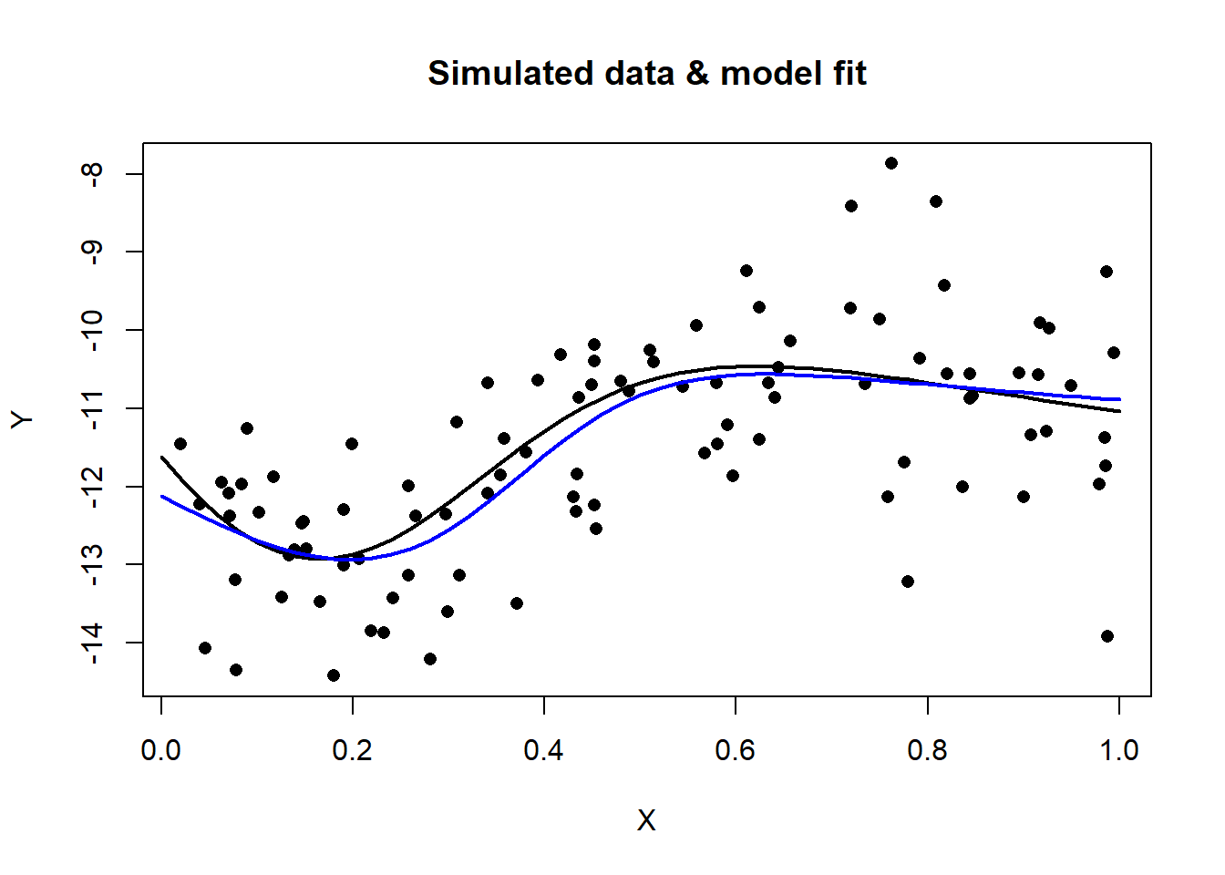
The training RMSE is returned by cfit_nn() and test RMSE can be found directly from the test data
# training RMSE
sqrt(fit$lossHistory[5000])
## [1] 0.9970785# test (expected) RMSE
yhat <- cpredict_nn(Xv, analysis_design, actFun=c(1, 0))
sqrt(mean((Yv[, 1] - yhat[, 1])^2))## [1] 1.018505The RMSE is an estimate of the residual standard deviation, which we know from the design of the simulation ought to be about 1.0.
It is almost impossible to draw any conclusions from a single set of training data, we do not know if, by chance, the simulation generated training data with some unusual feature. Clearly, we need to repeat the simulation with different seeds. For ease of presentation, I will create nine simulated sets of training data so that they fit into a 3x3 grid.
# The analysis design
arch <- c(1, 3, 1)
analysis_design <- cprepare_nn(arch)
# space for saving the performance measures
rmse_train <- rep(0, 9)
rmse_test <- rep(0, 9)
# seeds for the data and the starting values
set.seed(2503)
data_seed <- sample(1000:9999, size=9, replace=FALSE)
start_seed <- sample(1000:9999, size=9, replace=FALSE)
# run 9 simulations
par(mfrow=c(3,3))
for(i in 1:9) {
  # random set of training data
  set.seed(data_seed[i])
  X <- matrix(runif(100, 0, 1), ncol=1)
  Y <- cpredict_nn(X, base_design, actFun=c(1, 0)) + rnorm(100, 0, 1)
  # random starting values
  set.seed(start_seed[i])
  analysis_design$bias   <- runif(length(analysis_design$bias), -3, 3)
  analysis_design$weight <- runif(length(analysis_design$weight), -10, 10)
  # fit the analysis model
  fit <- cfit_nn(X, Y, analysis_design, eta=0.1, nIter=5000, trace=0, actFun=c(1, 0))
  # collect performance measures
  rmse_train[i] <- sqrt(fit$lossHistory[5000])
  yhat <- cpredict_nn(Xv, analysis_design, actFun=c(1, 0))
  rmse_test[i] <- sqrt(mean((Yv[, 1] - yhat[, 1])^2))
  # plot the data and fitted response
  Yf <- cpredict_nn(Xs, analysis_design, actFun=c(1, 0))
  plot(X[, 1], Y[, 1], pch=16, ylim=c(-14, -9), xlim=c(0,1), xlab="X", ylab="Y")
  lines(Xs[, 1], Ys[, 1])
  lines(Xs[, 1], Yf[, 1], col="blue", lwd=2)
}
mtext("Curves fitted to nine random datasets", side = 3, line = - 1.5,
      cex=1.5, outer = TRUE)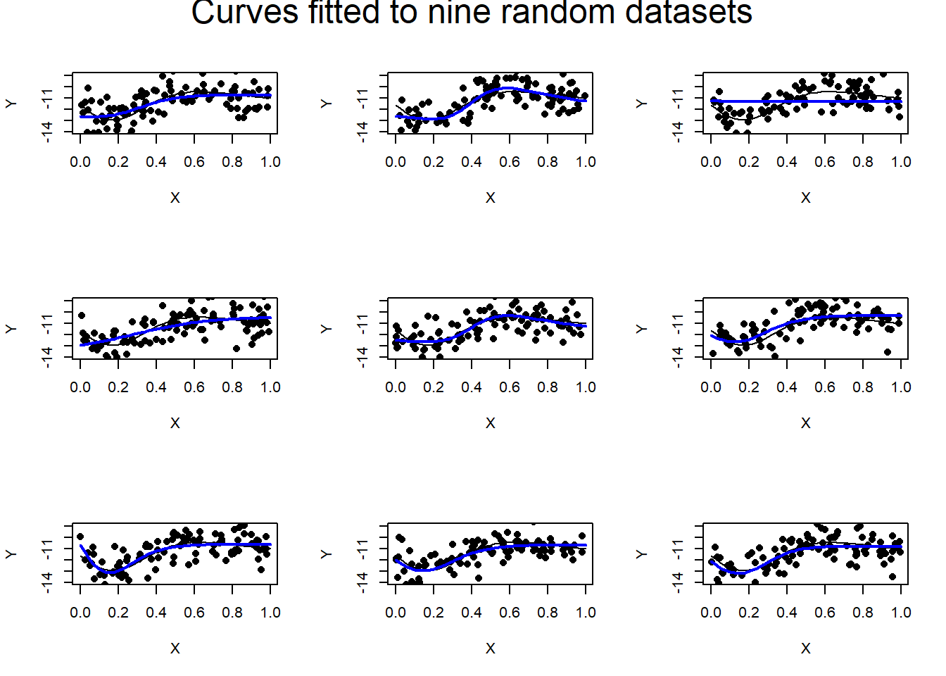
par(mfrow=c(1,1))
# summarise the performance measured
summary(rmse_train)
## Min. 1st Qu. Median Mean 3rd Qu. Max.
## 0.8914 0.9037 0.9417 0.9834 1.0174 1.2377summary(rmse_test)## Min. 1st Qu. Median Mean 3rd Qu. Max.
## 1.019 1.027 1.036 1.074 1.060 1.336Runs 3 and 4 completely fail to find the shape. Perhaps, more iterations would improve the performance, 5,000 was an arbitrary choice on my part; or perhaps it is the starting values. As is usual, the test RMSE is larger than the training RMSE indicating a slightly worse fit, but the difference is small.
Here is a second analysis of the same 9 datasets, but with different starting values.
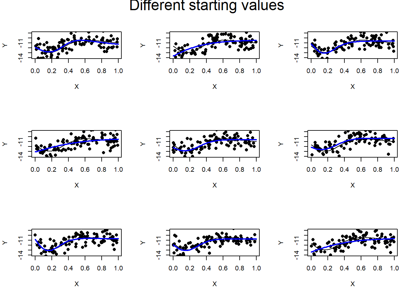
A nice example of the importance of repeating the gradient descent algorithm with different starting values. This time the model finds the curve for dataset 3 without a problem, but fails for datasets 2, 4 and 9.
Here is an analysis of the same basic curve but with N(0, 2) noise in the response.
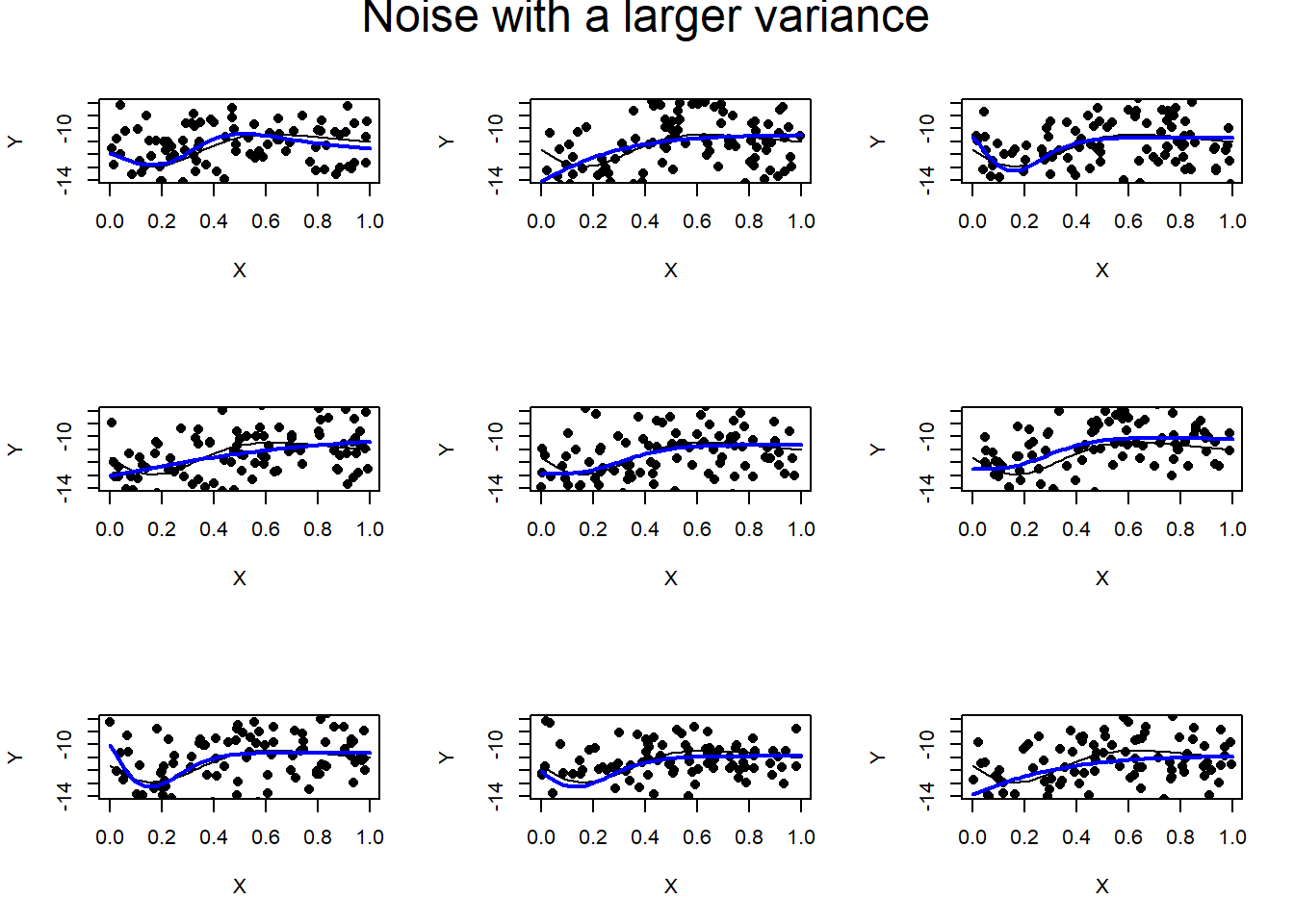
The underlying pattern is far harder to detect by eye and the analysis does well to recover it in four of the examples.
The experiment
I continued the investigation of fitting a NN(1, 3, 1) to this pattern of data by
- increasing the number of datasets to 20
- analysing each dataset 3 times from different starting values and taking the one with the lowest training loss
- varying the standard deviation of the noise, sigma, to be from 0.5 to 3.0 in steps of 0.5
- monitoring the training and test loss
This requires 20 x 3 x 6 = 360 analyses. Here are the results, averaged over the 20 datasets
| Investigation of the impact of increased noise | ||||
| averaged over 20 datasets | ||||
| Sigma | average RMSE | test-sigma | test/sigma | |
|---|---|---|---|---|
| training | test | |||
| 0.5 | 0.556 | 0.570 | 0.070 | 1.139 |
| 1.0 | 1.033 | 1.056 | 0.056 | 1.056 |
| 1.5 | 1.524 | 1.557 | 0.057 | 1.038 |
| 2.0 | 2.017 | 2.061 | 0.061 | 1.030 |
| 2.5 | 2.513 | 2.568 | 0.068 | 1.027 |
| 3.0 | 3.011 | 3.077 | 0.077 | 1.026 |
As the noise (sigma) increases, so the average test RMSE comes closer to sigma on the ratio scale (test/sigma), but further away as a difference (test-sigma). I was expecting a clear deterioration in performance as the standard deviation of the noise increases, but this not evident. One reservation that I have is that these fits come from the gradient descent algorithm run for exactly 5,000 iterations. As yet, I have not discussed the issue of a stopping rule, but we know from my previous post that if the algorithm is run for too long, the performance on test data will deteriorate. Perhaps, 5,000 iterations is too many when sigma=0.5.
Despite the simplicity of this investigation, it raises many questions that test our understanding neural networks and gradient descent.
- was 20 datasets enough?
- was 3 sets of starting values enough?
- ratio or difference, which is better? why?
- did the stopping rule have a distorting impact on the results?
- what would happen with even larger (smaller) amounts of noise?
- what about noise that is not Gaussian?
- would the same pattern be evident with a different underlying curve?
- are the results distorted by one or two datasets that are hard to fit?
- would we get the same pattern from a (1, 4, 1) neural network? what about other architectures?
- the data were generated by a NN(1, 10, 1), what would happen if that same architecture were used in the analysis?
A simulation with 5 predictors
In this simulation the data are generated from a (5, 6, 1) NN and analysed with a (5, 3, 1) NN. I have chosen to run 10,000 iterations to enable the gradient descent more time to search over the increased number of parameters.
Here is a single data set to help visualise the problem
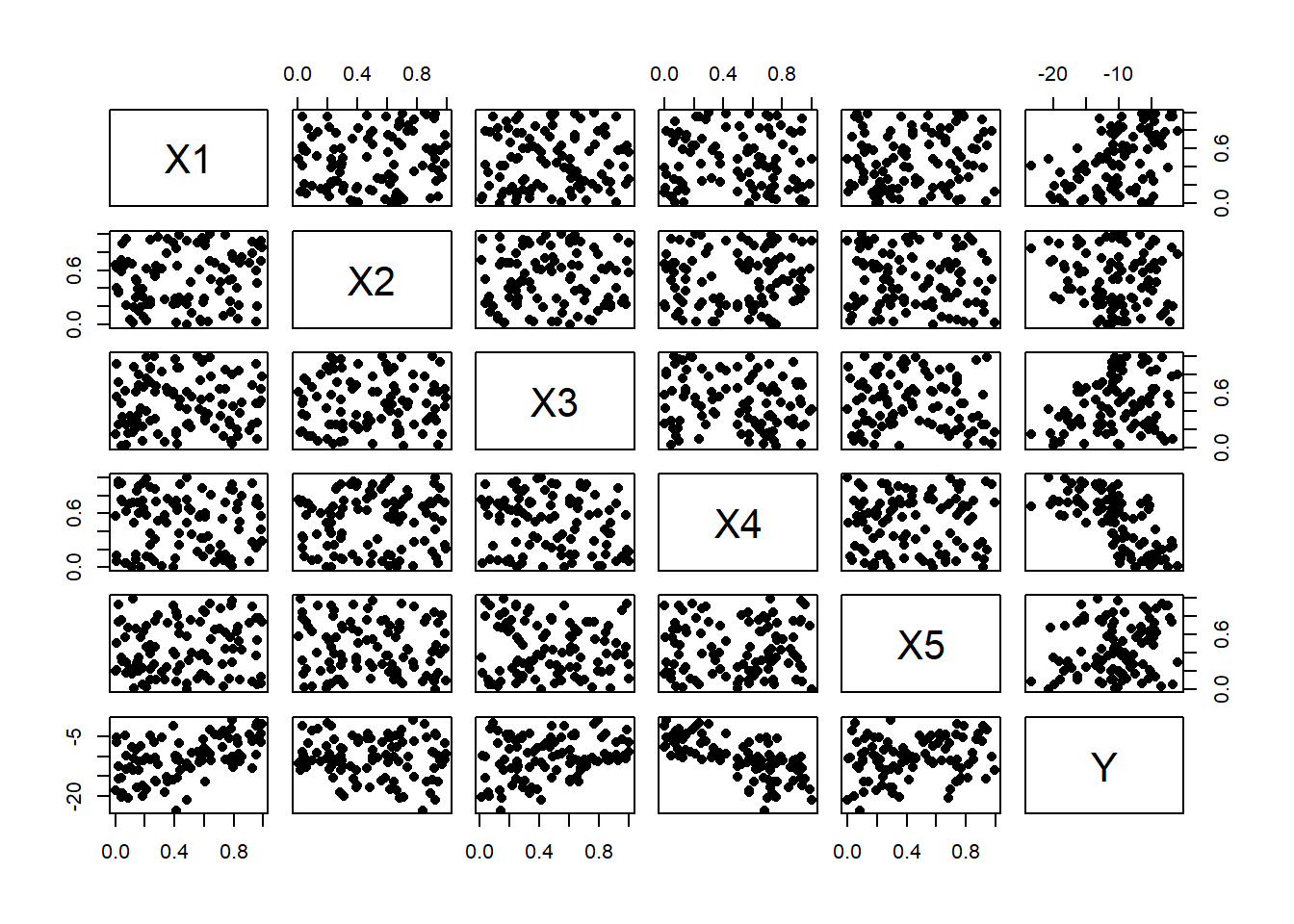
The Xs are independent uniform(0, 1) and the relationship with N is based on the NN plus N(0, 1) noise in the response.
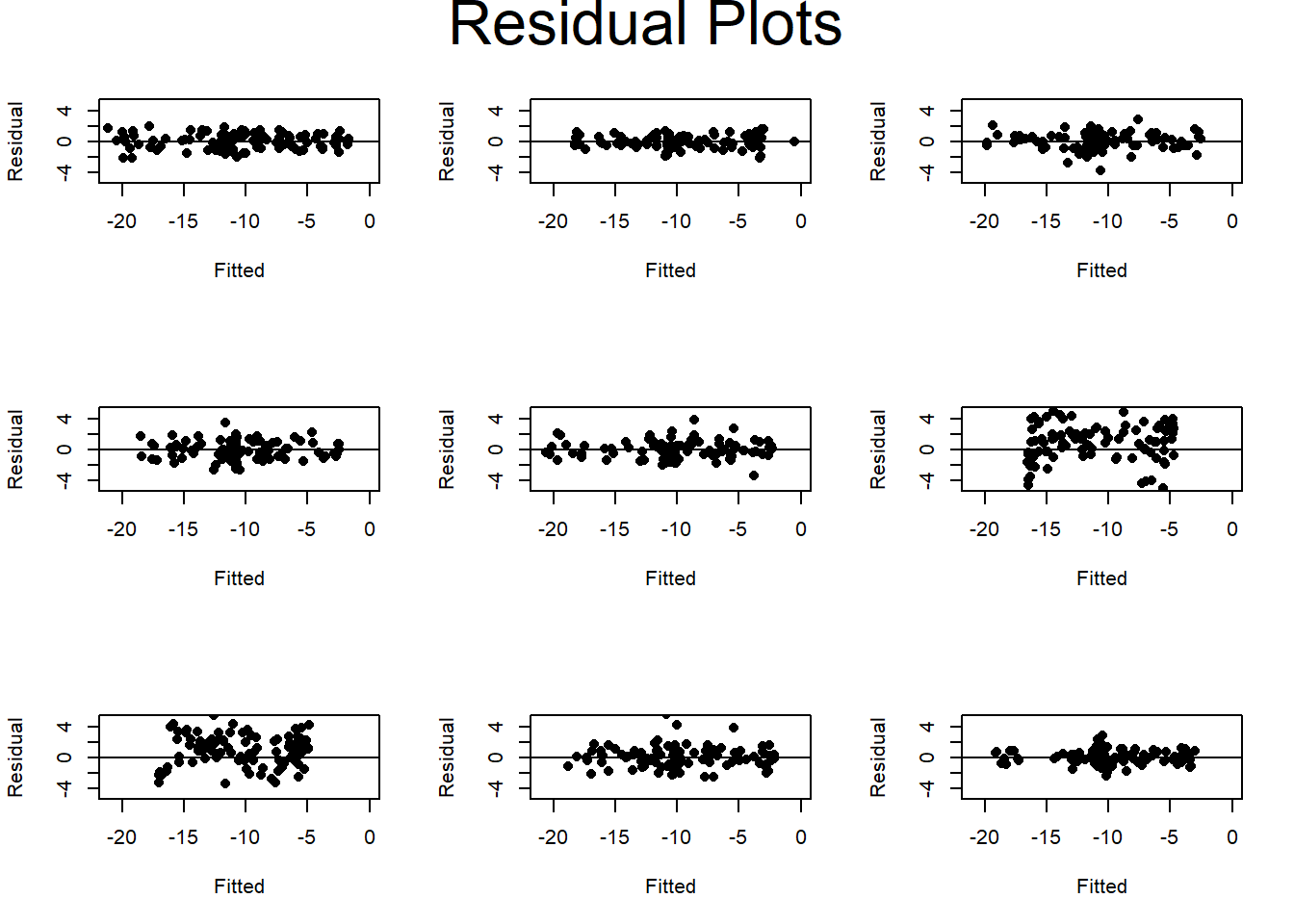
Here are the residual plots for 9 random datasets with the same underlying relationship
##    Min. 1st Qu.  Median    Mean 3rd Qu.    Max.
##  0.8417  1.0541  1.1566  1.3715  1.3620  2.4943
## Min. 1st Qu. Median Mean 3rd Qu. Max.
## 1.402 1.566 1.598 1.867 1.721 2.947The plots of residuals against fitted values show quite variable performance. Datasets 6 and 7 perform rather poorly. This can be seen in the training RMSEs that vary from 0.84 up to 2.49, when the ideal would be close to 1. Perhaps the algorithm needs more iterations, or maybe one set of starting values is insufficient. The test RMSE shows a similarly wide variation, but is always greater than 1.
Real Data
The advantages of using simulated data are clear, but they always leave you wondering if the methods that work well in a simulation experiment will also work well on real data. For this reason, it is good practice to take any workflow that is developed on simulated data and test it on real data.
One good source of real data is kaggle (https://www.kaggle.com/datasets). kaggle has a regular competition called playground in which they present smallish tabular datasets and invite people to try out their machine learning skills. These data are all based on real datasets, but the playground data are in fact simulated by deep learning to resemble the original data. In my experience the datasets are well-designed so as not to be too easy, but they always leave me wondering whether I am analysing the data, or the method that kaggle used in the simulation.
kaggle also offer a mass of real data some with prizes for the best solutions, but many others that are just there for interest. The problem is not the availability of data, but the difficulty of finding a dataset that is just right for your needs.
There is no point in listing the many other sources of real data, because there is already a Wikipedia page that does the job https://en.wikipedia.org/wiki/List_of_datasets_for_machine-learning_research
Google even has a search engine specifically designed for finding datasets https://datasetsearch.research.google.com/
If your interests are scientific then Nature has a useful webpage at https://www.nature.com/sdata/policies/repositories that lists relevant data repositories. The data in these repositories are often linked to scientific publications. I have found the Dryad repository (https://datadryad.org/search) and the GEO repository (https://www.ncbi.nlm.nih.gov/geo/) to be particularly useful.
Half and half
When there is a particular real dataset or a particular real type of data that are of special interest, a good plan is to base the simulation study on those real data. Such simulations can be controlled by unsupervised neural networks as, I assume, kaggle does for its playground series, but such neural networks require quite a lot of development beyond what I have covered so far, so I will need to return to this approach at a later date.
How many replicates
In my examples, I have chosen to run nine replicate datasets, because they plot neatly in a 3x3 grid. Generally you will need more than nine replicates.
The key to making the choice of the final number of replicates is to base it on a preliminary run with just a few replicates. Take the example with 5 predictors given above. The mean test RMSE was 1.9 and the standard deviation was about 0.5. This means that the standard error of the mean was about 0.5/sqrt(9) or 0.17 and the true average test RMSE is likely to be between 1.56 and 2.24 (two standard errors from the mean). This is a very wide range, which would make comparison with other methods very unreliable.
Suppose that you decided that you needed to know the true test RMSE to within 0.2 i.e. a standard error of 0.1. The formula, 0.5/sqrt(n)=0.1 implies that n=25, so we would need to run 25 replicate sets of data.
You could extend such back of the envelope calculations into a full analysis of power as you might when designing a clinical trial or a real world experiment. This is probably over the top. If you run insufficient replicates then it will be evident when you look at the results, in which case you just redesign the experiment and run it again. Simulation experiments are cheap, at least for small to moderate sized neural networks.
Conclusions
Neural networks with random weights and biases provide an excellent way of creating simulated datasets with a variety of underlying structures. In any experiment based on simulation from a NN, it is good practice to include one analysis based on the the same architecture as was used in the simulation, as this will form a baseline against which other models can be compared. However, good performance when you have the true model is of no real importance in itself, since real data are not generated by a NN and if they were, you would not know the underlying truth. Justifying the choice of network architecture for the analysis is one of the main jobs of a comprehensive workflow.
Appendix: Code Changes
The C code used in this and my previous post can be found on my GitHub pages (https://github.com/thompson575/NeuralNetworks) as cnnUpdate01.cpp.
When simulating data from a NN it is useful to be able to switch off the activation for one of the hidden layers so that that layer can be used as the predictors while the output layer is the response. To enable this I modified the code so that the activations are given as a coded vector with one value for each layer and the different activations are built into a single C function. Here is a simplified version of the C function
double cActivation(double z, int actFun = 0) {
  switch( actFun ) {
  case 1:
    return 1.0 / (1.0 + exp(-z));
  default:
    return z;
  }
}
A data generating (2, 6, 5, 6, 1) neural network might have activation c(1, 0, 1, 0). The input layer does not need an activation function, so this coded vector says that the first hidden layer of 6 nodes uses the sigmoid, then next with 5 nodes uses the identity, then then sigmoid again and the output layer uses the identity. The other advantage of this rewriting of the code is that it will be easy to add other activation functions.
A new function cNodalValues() takes a set of weights and biases and a set of input values and returns the calculated values for every node. This extends cpredict_nn() that does the same thing but only returns the output layer. This function is useful for extracting an internal hidden layer when simulating.