Neural Networks: Search Paths
Introduction
In my last post, I described C code for fitting neural networks by gradient descent and explained how that code can be incorporated into R using the Rcpp package. Now, I want to consider how that gradient descent algorithm works.
I find it easier to understand concepts if I can represent them in a diagram, so I base this discussion on my preferred visualisation of the search paths of gradient descent. I believe that this diagram is helpful in understanding many of the ideas behind machine learning and I will use it again when I cover topics such as over-fitting, cross-validation and regularization.
Current and Future Performance
Think of a model as a machine \(f_\theta(X)\) for making predictions of a response Y. Here X represents the measured features, f() is the general form of the model and \(\theta\) is the set of model parameters.
The performance of the model on training data {\(X_T, Y_T\)} is measured by the value of some chosen loss function.
\[ \text{Training loss} = Loss(Y_T, f_\theta(X_T)) \]
The loss measures the distance between the true response and its prediction.
The plan is to use the model to predict response Y for as yet unknown data, X, which is independent of the training data but from the same source. The best measure of the performance of the model on new data is the average or expected loss over all possible sets {X, Y}.
\[ \text{Expected Loss} = E_{X,Y} \left\{ Loss(Y, f_\theta(X)) \right\} \]
The new data {X, Y} may not have the same number of observations as {\(X_T, Y_T\)} so to make the training loss and the expected loss comparable, the loss is scaled as loss per observation. This means that we can create a very good approximation to the expected loss by taking a single large test dataset {X, Y} and calculating
\[ \text{Test Loss} = Loss(Y, f_\theta(X)) \approx \text{Expected Loss} \]
The training loss measures performance of the model on one specific dataset and is of limited interest, while the expected loss measures the average performance across all new data and is the best indicator of the worth of the model. It is the expected loss that needs to be minimised.
In practice, the training loss can be calculated directly, but it is unlikely that data will exist to enable calculation of the expected loss, since it is rare to have large amounts of test data from the same source as the training data. One situation in which the expected loss can be calculated is in a simulation study. As we will see later in this post, any amount of test data can be simulated using the same model as was used to create the training data.
Picturing the Model Fitting
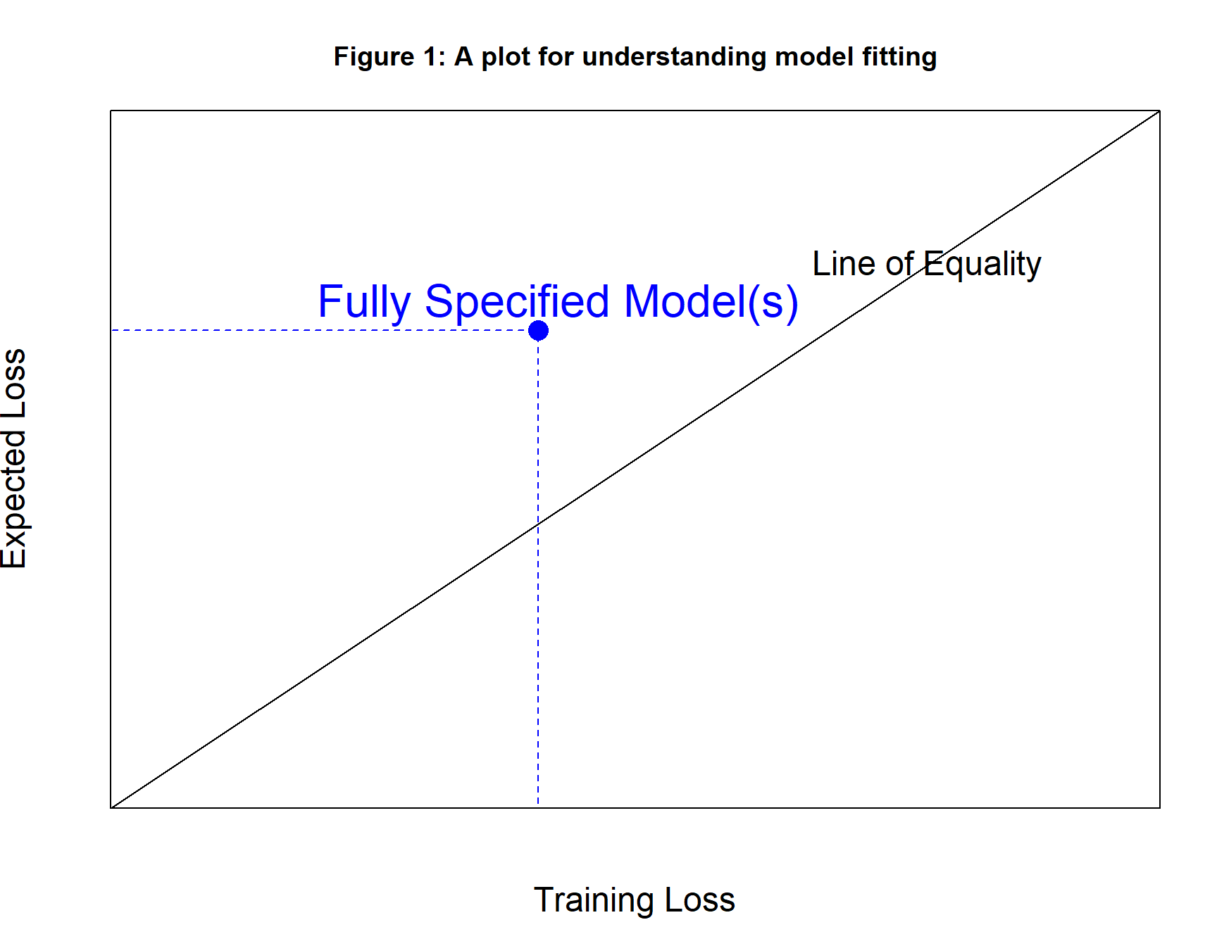
Figure 1 shows the diagram that I use to understand model fitting. It takes the form of a plot of the training loss per observation (x-axis) against the expected loss per observation (y-axis).
Think of the expectation of the loss for a given model and given data source as fixed but unknown, while the training loss depends on the particular training sample that is used and can be calculated exactly. In practice, the expected and training loss of a specified model should be similar, because they are defined on data from the same source. We can think of the training loss as an estimate of the expected loss.
Every possible model with known parameter values has both a training loss and an expected loss, so every model can be plotted as a point on the diagram. It is possible that two models with different parameter values will have the same training loss and the same expected loss, so a single point on the plot might equate to multiple models.
The Ladder of Models
Figures 2 and 3 show what I call the ladder of prediction models. Let’s consider the four steps in this ladder.
Level 0: The Perfect Model
Suppose that you wanted to predict my height, y. All you know about me is \(x\)={male, biostatistician, lives in UK}, so I doubt that your prediction will be very accurate. However, we can imagine having complete information, \(x^c\), which would include my genome, the history of every meal that I have ever eaten, every illness etc. You would also need to know how to use this complete information, which is to say, a function \(G(x^c)\) that predicts y with total accuracy.
A loss function, \(L()\), is chosen to measure the average difference between the real response, \(y\), and the prediction, \(G(x^c)\), over a set of subjects i=1,…,n. \[ \frac{1}{n} \sum_{i-1}^n L(y_i, G(x^c_i)) = 0 \] Since the predictions are always perfect this loss will be zero regards of the selection of subjects, so both the expected and the training loss will be zero.
Level 1: The Ideal Model
Unfortunately, you have \(x\) and not \(x^c\), but there will be a model, \(g()\), that makes the best possible use of x, that is to say, it minimises the expected loss. Predictions are no longer perfect, so the value of the loss over a sample of subjects will vary from sample to sample. None the less, the expected loss, which is averaged over all possible samples, will be fixed and as small as it can be without more features.
Level 2: The Best Model
Unfortunately, you do not know the functional form of \(g()\), so you are forced to pick a flexible function \(f_\theta()\) that changes its shape depending on parameters \(\theta\). The hope is that by choosing the parameters carefully, you will be able to make \(f_\theta(x)\) close to \(g(x)\). Let’s call the optimal choice of parameters \(\Theta\).
The loss in a sample of size n will be, \[ \frac{1}{n} \sum_{i-1}^n L(y_i, f_\Theta(x_i)) \] For very large n, this approximates the expected loss, but the training set will usually have much smaller size and its loss will vary randomly about the expected value. The Best Model (for this family) should lie reasonably close to the line of equality on the diagram.
Level 3: The Fitted Model
Unfortunately, you do not know the optimal values of the parameters \(\Theta\), so you are forced to make a reasonable guess \(\hat{\theta}\), which you do based on the training data and your favourite algorithm. The fitted model is \(f_\hat{\theta}(x)\).
You want the expected loss based on \(\hat{\theta}\) to be as close as possible to the expected loss based on \(\Theta\). Most algorithms select \(\hat{\theta}\), because those parameters gives a low training loss, so usually the fitted model lies above the line of equality where the training loss is less than the expected loss.
Representing the ladder of models
Figure 2 represents the four steps in the ladder of models. The perfect model (purple) has zero training loss and zero expected loss, but it requires complete data, which we do not have. The ideal model (green) uses the available predictors is the optimal way, but we do not know what model is optimal, so we select a flexible family of models as represented by the red parabolic shape. The best model (red) is the member of this family with the minimum expected loss. Sadly, we do not even know the combination of parameters needed to define the best model, so we have to fall back on a fitted model (dark blue).
In this figure, the possible combinations of training and expected loss for the chosen family of models with different parameters define a regular parabolic shape. This is purely diagrammatic, for complex models the shape could be highly irregular,
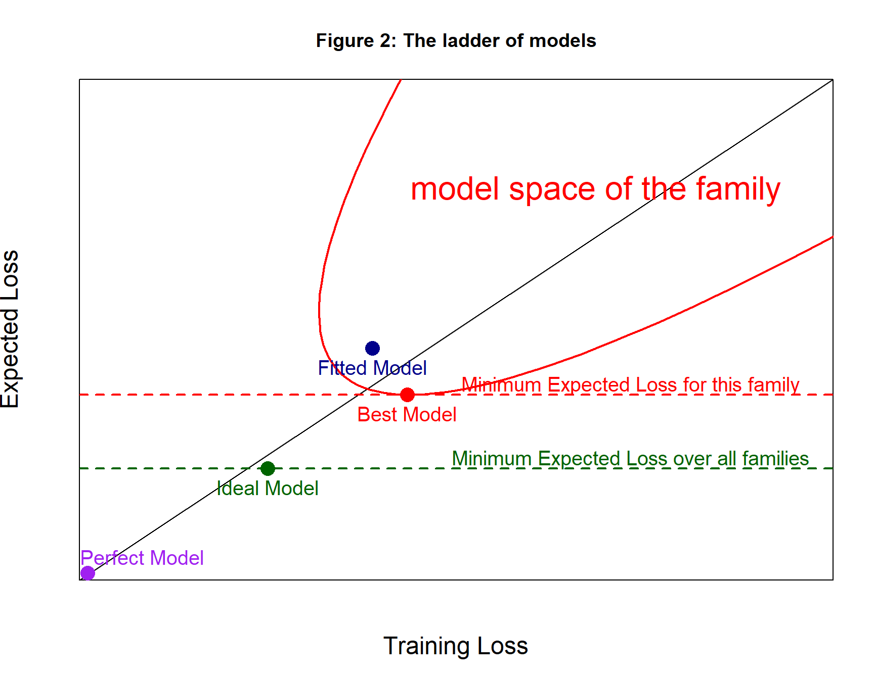
Why is the best model in figure 2 to the right of the line of equality? This is just the luck of the draw. We have a single random set of training data and as figure 2 is drawn, it so happens that the training sample has a relatively high loss.
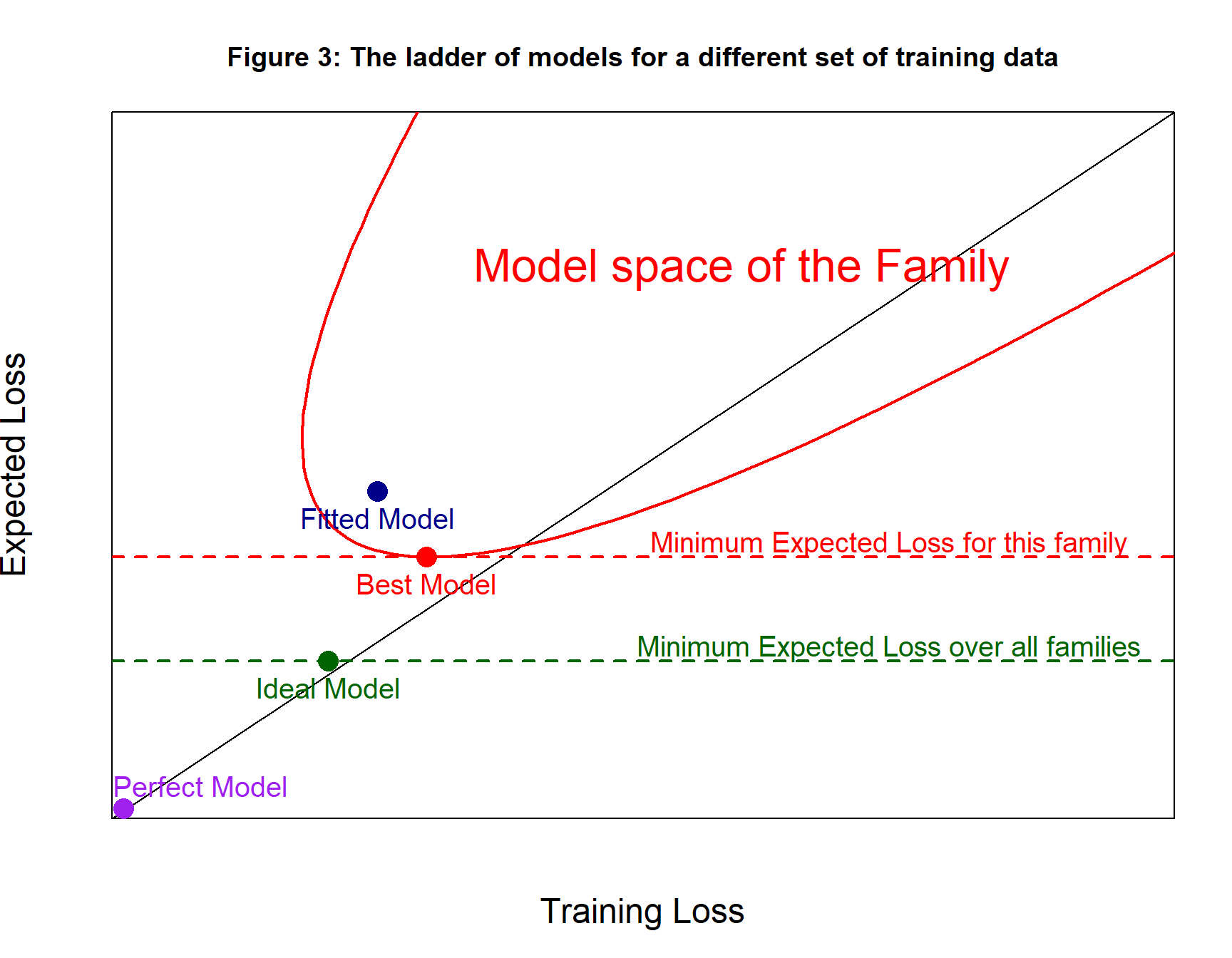
Draw a different set of training data and the area defined by the family might move to the left. All models have the same expected loss regardless of the training data, so models move to the left or right when the training data change, but they stay parallel to the x-axis. Not every model moves to the same extent; a model that does relatively well on one training set may do less well on others. It is not a rigid movement of the area to the left with all models keeping their relative position.
Of course, the best model has exactly the same parameters, because it is defined by the expected loss and does not depend on the training data. Figure 3 shows the same diagram as figure 2, but for different training data.
Search Paths
Fitting a neural network involves choosing random starting values for the parameters and then adjusting them in small steps based on the gradient of the training loss. These small improvements correspond to a series of steps to the left in figure 4. The algorithm will stop when it reaches a local minimum in the training loss, or when it finds the global minimum, or when the user tells the algorithm to stop early.
In figure 4, the path taken by the algorithm is shown as a brown dashed line and the point along the path with the minimum expected loss is shown as a dark green point. This is the fitted model and represents the best of the models visited by the algorithm.
We live in the hope that the search path will pass through, or close to, the Best Model with its minimum expected loss, but this is just a hope.
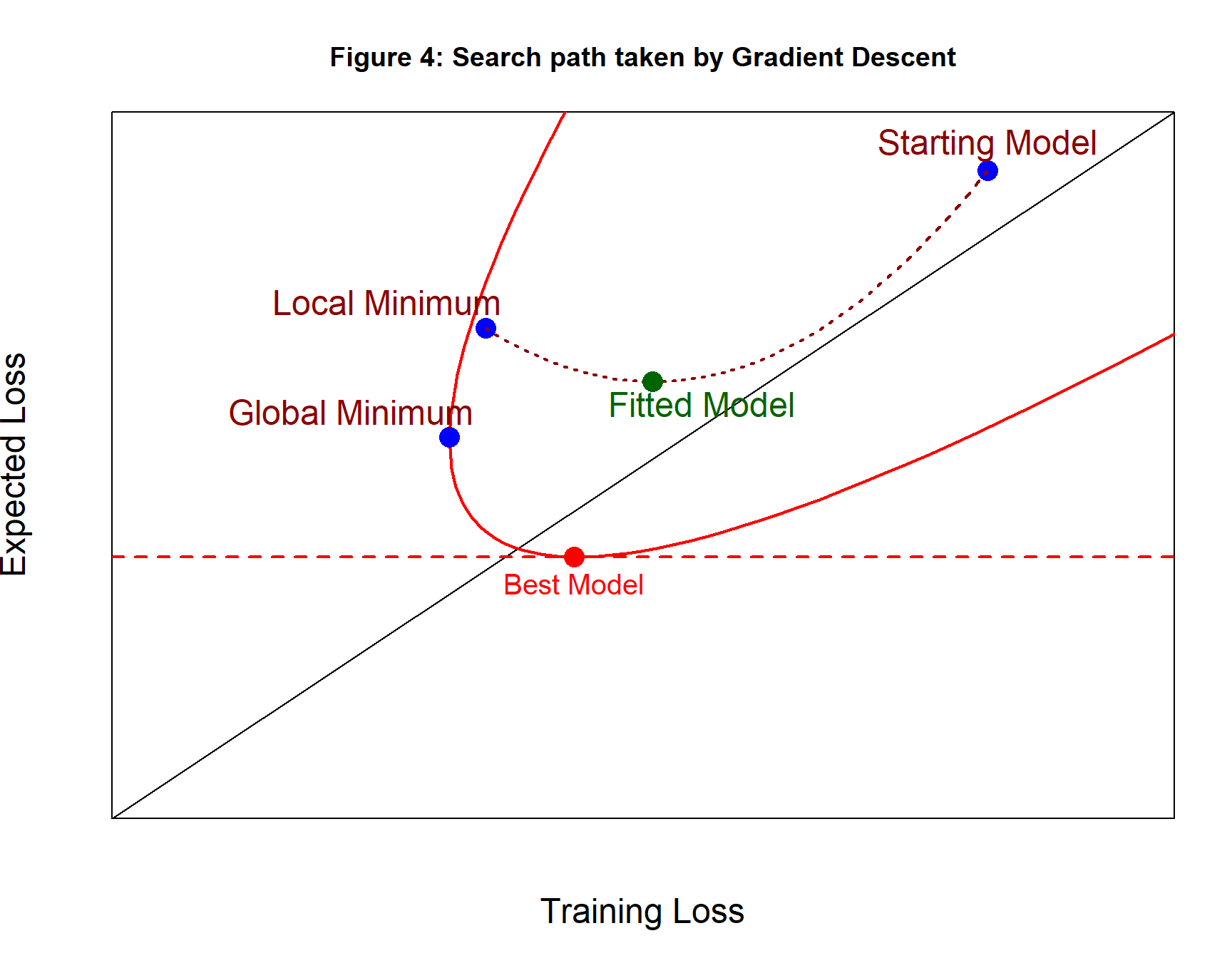
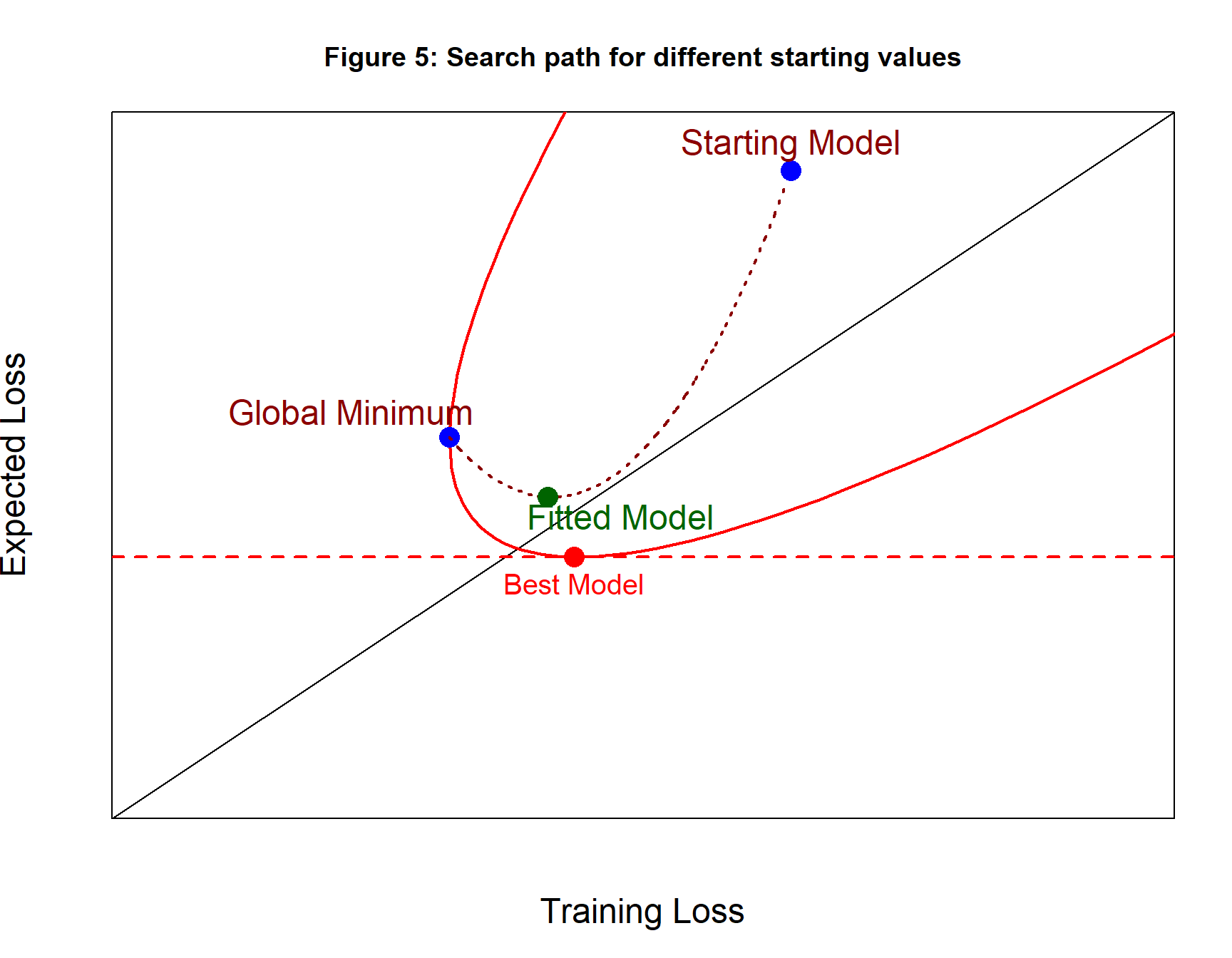
Figure 5 shows a second search path with different starting values that ends with the global minimum. Converging to the global minimum of the training loss does not guarantee that the path will pass close to the best model.
Remember that this is just a diagram, the search paths might not be as smooth and regular as the ones shown in figures 4 and 5.
It is common practice to draw two separate curves to show the progress of the algorithm from iteration to iteration, one curve for the training loss and one for the expected loss (or some approximation to it). Figure 6 shows such a plot using exactly the same values as those used to generate figure 5.
For this example, the fitted model is found at iteration 320 of the algorithm.
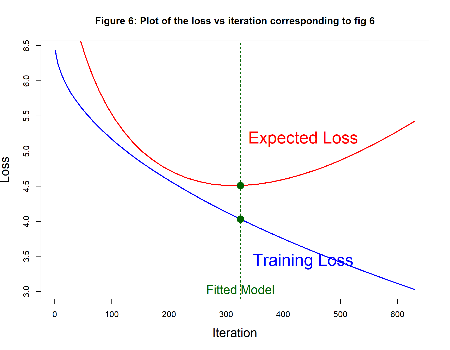
Whichever plot is drawn, when the fitted model is chosen based on the minimum of the expected loss estimated from a second (validation) dataset, that estimate of the expected loss will tend to exaggerate the true future performance. A third (test) sample would be needed to give a more reliable estimate. When the validation sample is very large, this bias should be small.
Increasing the size of the training set
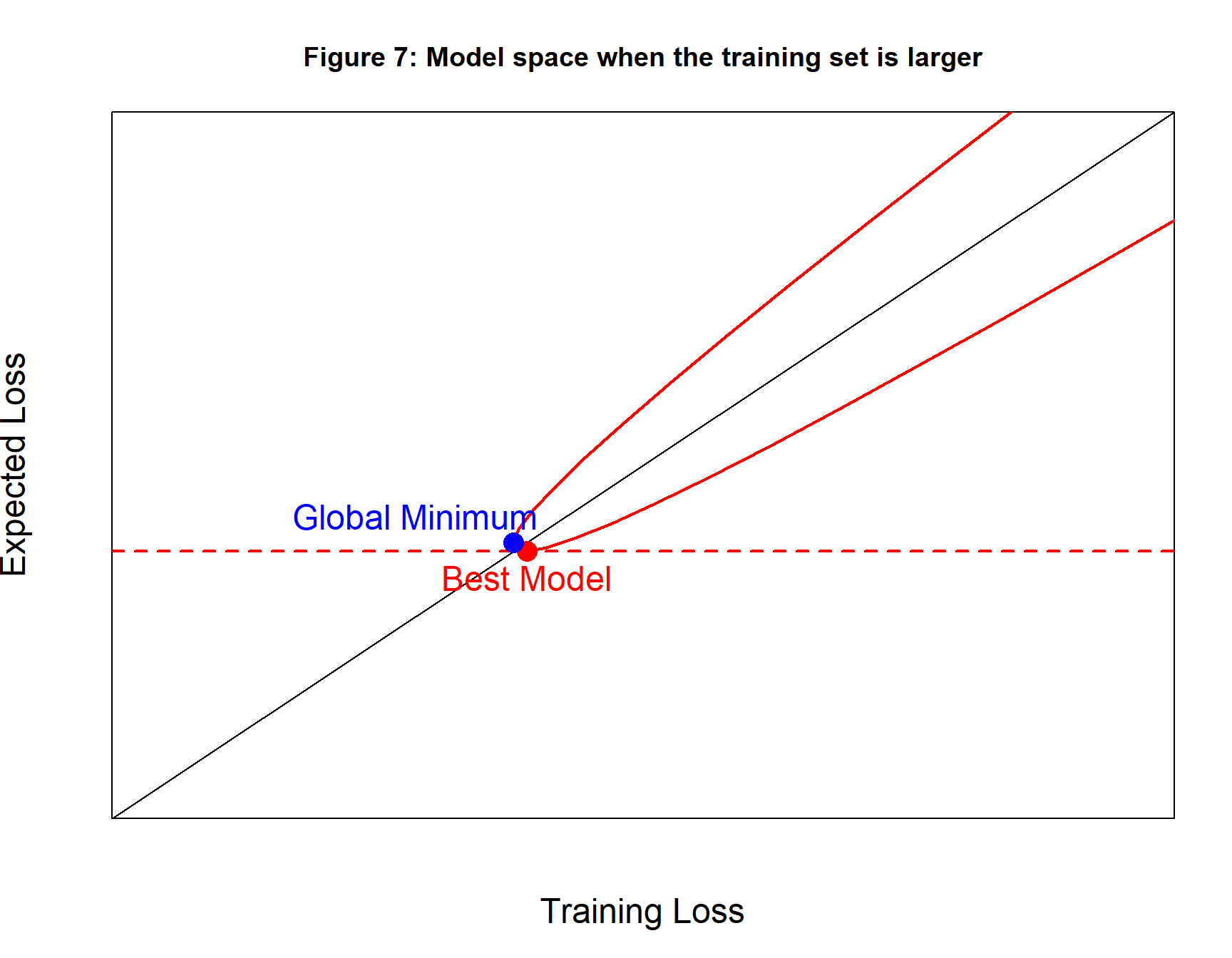
We can increase the chance that the global minimum of the training loss will have a low expected loss by making the training data more representative and the way to do this is to increase the size of the training set. As figure 7 shows, this would make the area defined by the family narrower and closer to the line of equality. The chance that the training loss is very different from the expected loss is reduced.
A simulated example
Figure 8 shows a training set of 100 observations that vary randomly about a bell-shaped Gaussian curve. The random noise in the simulation has a standard deviation of one, so we would expect a well-fitting model to have a RMSE that is close to one.
This example requires a new C function that monitors the loss in the test data as well as the loss in the training loss. The additions to my C code are described in an appendix at the end of this post.
set.seed(9293)
X <- matrix( runif(100), ncol=1)
Y <- matrix( 5 * exp( -20*(X[, 1]-0.6)^2) + rnorm(100, 0, 1))
xp <- seq(0, 1, 0.01)
yp <- 5 * exp( -20*(xp-0.6)^2)
plot(X[, 1], Y[, 1], pch=16,
     xlab="X", ylab="Y", main="Figure 8: Training data n=100")
lines(xp, yp, lwd=2, col="blue")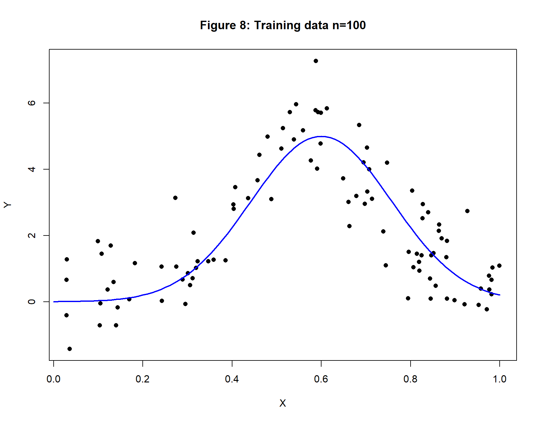
A large test dataset with n=10,000 will be used to estimate the expected loss.
XV <- matrix( runif(10000), ncol=1)
YV <- matrix( 5 * exp( -20*(XV[, 1]-0.6)^2) + rnorm(10000, 0, 1))
xp <- seq(0, 1, 0.01)
yp <- 5 * exp( -20*(xp-0.6)^2)
plot(XV[, 1], YV[, 1], pch=16,
     xlab="X", ylab="Y", main="Figure 9: Test data n=10,000")
lines(xp, yp, lwd=2, col="blue")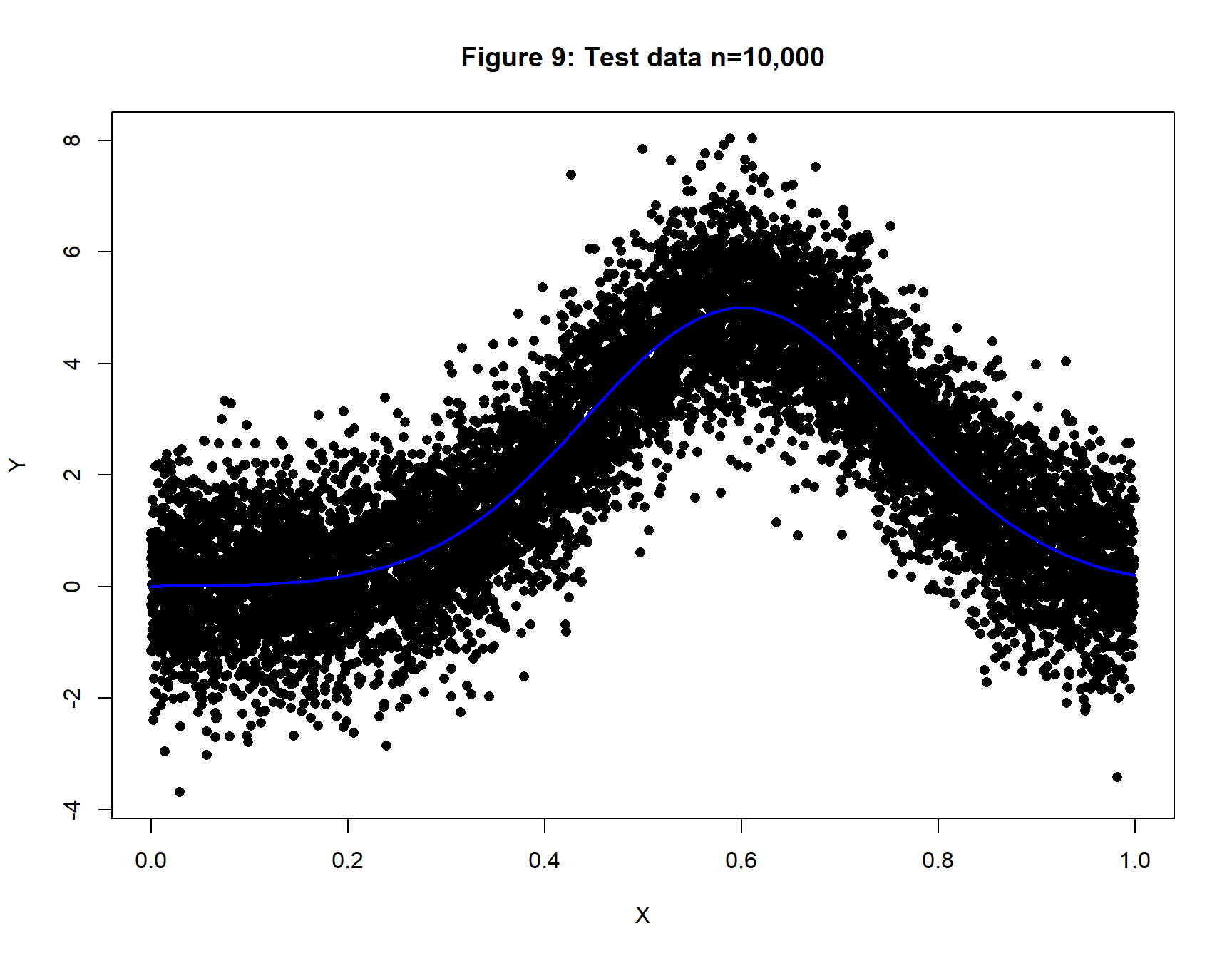
Analysis 1: A (1, 4, 1) Neural Network
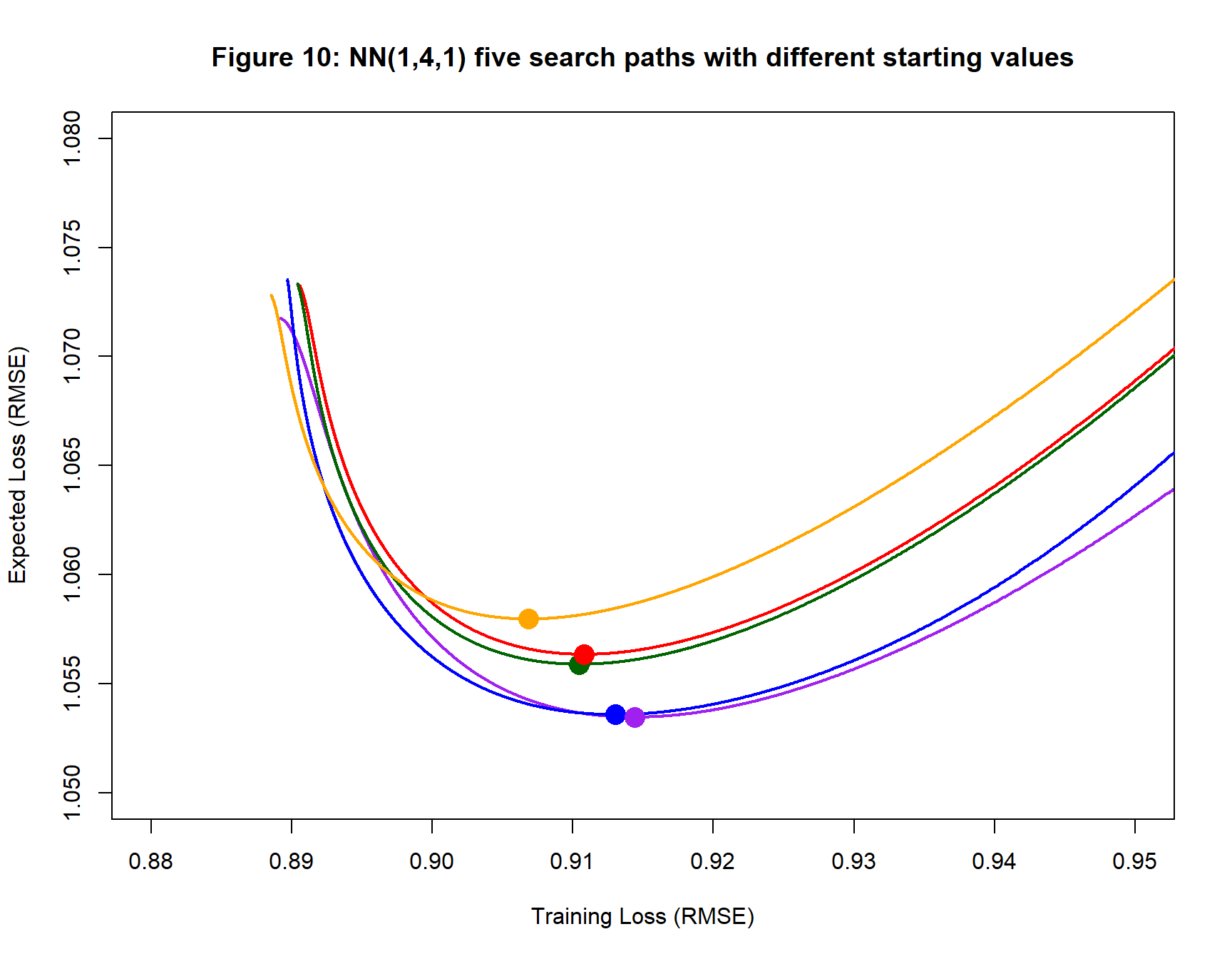
My first analysis models the training data using the family of neural networks that have one input, 4 hidden nodes and 1 output. The gradient descent algorithm is run five times on the same training data with different randomly chosen starting values. The algorithm uses a sigmoid activation function for the hidden layer, a learning rate (step length) of 0.1 and is run for 10,000 iterations. Performance is assessed using the RMSE loss function.
Figure 10 shows the five search paths. The paths start well to the right of then area shown and progress leftwards to the fitted models, which are shown as coloured dots. After reaching the fitted models the search paths continue to reduce the training loss, but the expected loss increases.
| Table 1: Neural Network (1, 4, 1) | |||||||
| Details of the Fitted Models | |||||||
| Colour | Iteration | Loss (RMSE) | Weights | Biases | |||
|---|---|---|---|---|---|---|---|
| Training | Expected | mean | std | mean | std | ||
| Purple | 1635 | 0.914 | 1.053 | 1.95 | 7.64 | −0.40 | 4.77 |
| Blue | 2258 | 0.913 | 1.054 | −2.12 | 7.32 | 2.47 | 3.30 |
| Red | 2325 | 0.911 | 1.056 | 2.76 | 7.11 | −4.21 | 2.77 |
| Dark Green | 2013 | 0.910 | 1.056 | 3.20 | 6.93 | −2.39 | 4.85 |
| Orange | 2281 | 0.907 | 1.058 | −0.70 | 8.23 | 0.33 | 4.95 |
| Average | 2102 | 0.911 | 1.055 | 1.02 | 7.45 | −0.84 | 4.13 |
Points to notice
- The fitted models all have Expected losses (RMSEs) slightly above 1. The RMSE of the Ideal model (a Gaussian) is 1.0, so the Best Model must be close to Ideal.
- The expected losses of the fitted models are similar. They differ by a maximum of 0.007, which is 6.6% of their average
- The Expected loss of the Best Model must be less than 1.053 (purple path), the consistency of the five paths gives us hope that the best expected loss will not be far from 1.053, but it is just hope.
- No two sets of starting values lead to the same fitted model.
- The training loss at convergence (in this case after 10,000 iterations) has no relation to the actual performance of the model.
- It is important to re-run any gradient descent analysis with different starting values.
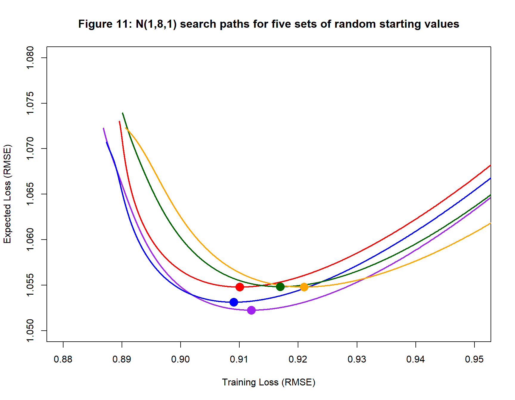
In figure 11 the orange path crosses the other paths. When search paths cross, it might be supposed that the two paths have reached the same model, that is to say, neural networks with the same weights and biases, but this is not so. The paths cross when a model on one path has the same training and expected loss as a model on the other path, but having the same losses does not imply that the weights and biases are the same. Two quite different models can have the same losses, especially when the model is over-parameterised. Had the models been identical, they would have had the same gradients and after coming together they would have continued along the same path. This clearly does not happen.
Analysis 2: A (1, 8, 1) Neural Network
Next, a (1, 8, 1) neural network is fitted to the same training data. The form of the gradient descent algorithm is kept the same. The resulting search paths are shown in figure 11 with the fitted models summarised in table 2. The fitted models have very similar performance to those found in the (1, 4, 1) analysis, but perhaps the training losses of the fitted models are slightly larger.
| Table 2: Neural Network (1, 8, 1) | |||||||
| Details of the Fitted Models | |||||||
| Colour | Iteration | Loss (RMSE) | Weights | Biases | |||
|---|---|---|---|---|---|---|---|
| Training | Expected | mean | std | mean | std | ||
| Purple | 1925 | 0.912 | 1.052 | −0.36 | 5.79 | 1.96 | 3.81 |
| Blue | 2288 | 0.909 | 1.053 | −1.30 | 5.72 | 1.34 | 4.01 |
| Red | 2037 | 0.910 | 1.055 | −0.56 | 5.38 | 0.25 | 4.22 |
| Dark Green | 1499 | 0.917 | 1.055 | 1.84 | 5.35 | 0.57 | 3.98 |
| Orange | 1713 | 0.921 | 1.055 | 1.73 | 5.44 | −1.38 | 4.14 |
| Average | 1892 | 0.914 | 1.054 | 0.27 | 5.54 | 0.55 | 4.03 |
Analysis 3: A (1, 16, 1) Neural Network
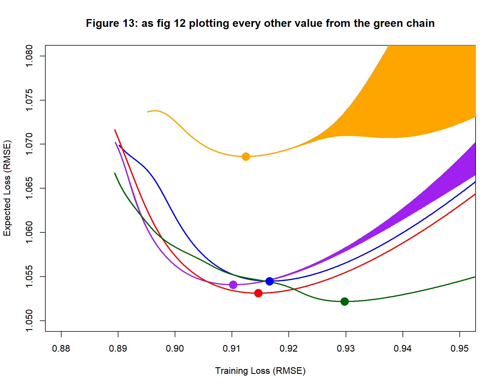
Next, the data are analysed using a (1, 16, 1) neural network. Everything else is kept the same. The resulting search paths are shown in figure 12. The search paths show wide oscillations in the losses along the search path leading to the blocked out appearance.
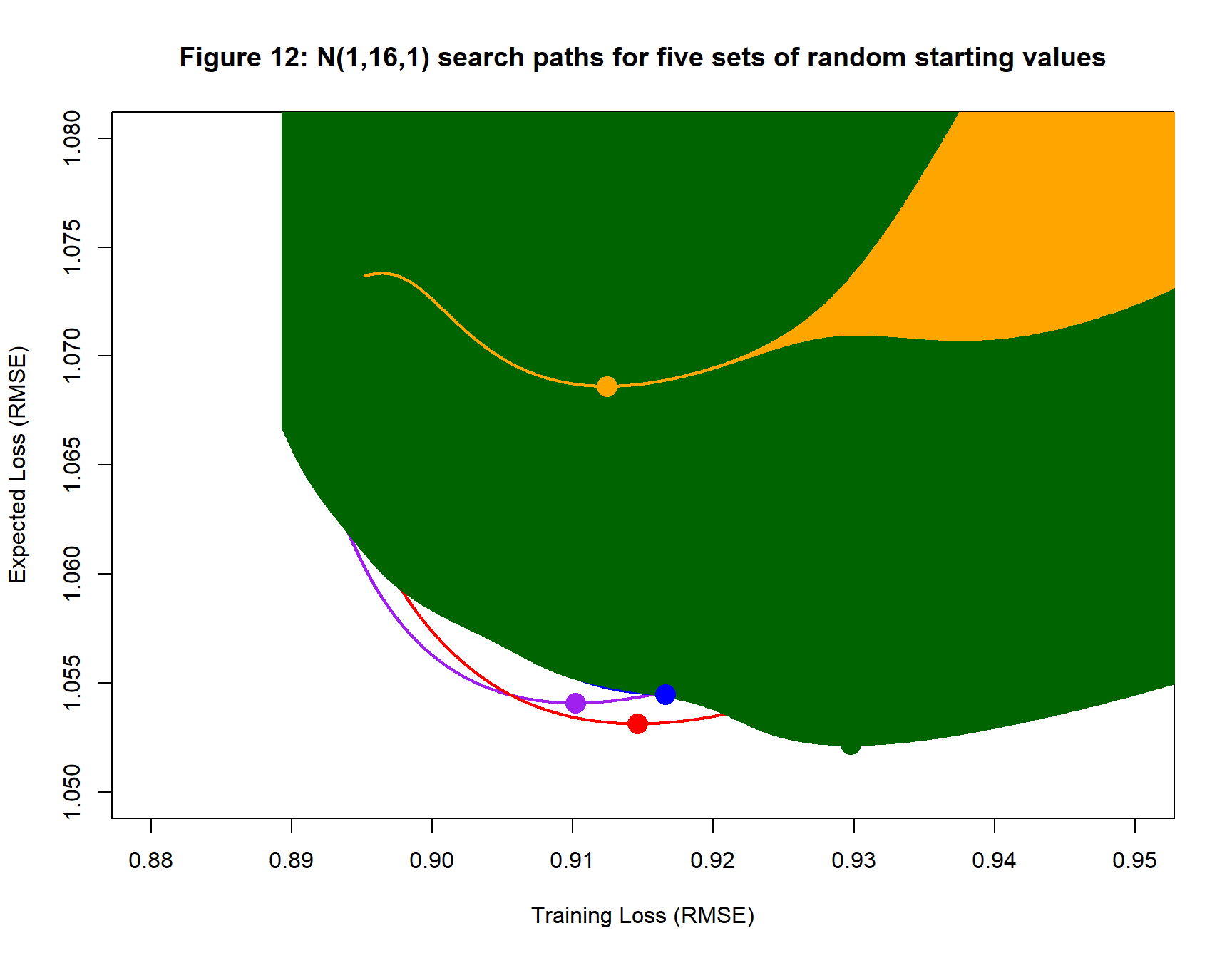
Since so much of the detail in figure 12 is obscured by the oscillation in the green path, I have replotted it showing only alternate iterations of the algorithm so that figure 12 shows the lower boundary of the green region. The oscillation in the orange and purple paths is now evident.
It is clear that the orange path produces a fitted model that is very different to the others, even though the training loss of the orange fitted model is similar. This difference is also clear from the values in table 3.
| Table 3: Neural Network (1, 16, 1) | |||||||
| Details of the Fitted Models | |||||||
| Colour | Iteration | Loss (RMSE) | Weights | Biases | |||
|---|---|---|---|---|---|---|---|
| Training | Expected | mean | std | mean | std | ||
| Purple | 2801 | 0.910 | 1.054 | 0.66 | 4.76 | 0.24 | 4.02 |
| Blue | 2304 | 0.917 | 1.054 | 0.76 | 4.48 | −0.86 | 3.59 |
| Red | 2244 | 0.915 | 1.053 | 0.12 | 4.39 | −0.73 | 3.66 |
| Dark Green | 2681 | 0.930 | 1.052 | −0.36 | 4.76 | 0.75 | 3.90 |
| Orange | 4403 | 0.912 | 1.069 | 0.48 | 4.59 | −0.30 | 3.97 |
| Average | 2887 | 0.917 | 1.056 | 0.33 | 4.60 | −0.18 | 3.83 |
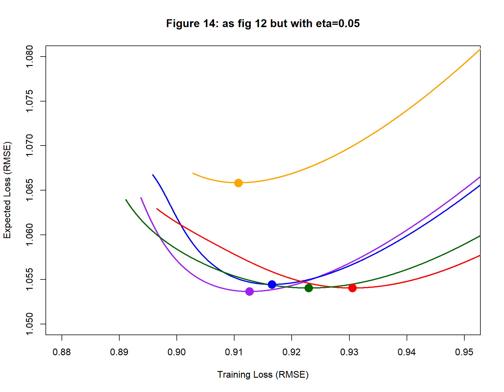
To show that the oscillation is a result of step length, I re-fit the (1, 16, 1) network using a step length, eta, of 0.05. The new results are shown in figure 14 and table 4. The orange search path still performs much worse than the others, but there is no longer any oscillation.
| Table 4: Neural Network (1, 16, 1) eta=0.05 | |||||||
| Details of the Fitted Models | |||||||
| Colour | Iteration | Loss (RMSE) | Weights | Biases | |||
|---|---|---|---|---|---|---|---|
| Training | Expected | mean | std | mean | std | ||
| Purple | 5179 | 0.913 | 1.054 | 0.73 | 4.74 | 0.48 | 3.87 |
| Blue | 4605 | 0.917 | 1.054 | 0.78 | 4.51 | −0.76 | 3.61 |
| Red | 4457 | 0.931 | 1.054 | 0.28 | 4.38 | −0.27 | 3.46 |
| Dark Green | 4072 | 0.923 | 1.054 | −0.24 | 4.70 | 1.33 | 3.57 |
| Orange | 8295 | 0.911 | 1.066 | 0.44 | 4.56 | 0.29 | 3.92 |
| Average | 5322 | 0.919 | 1.056 | 0.40 | 4.58 | 0.22 | 3.68 |
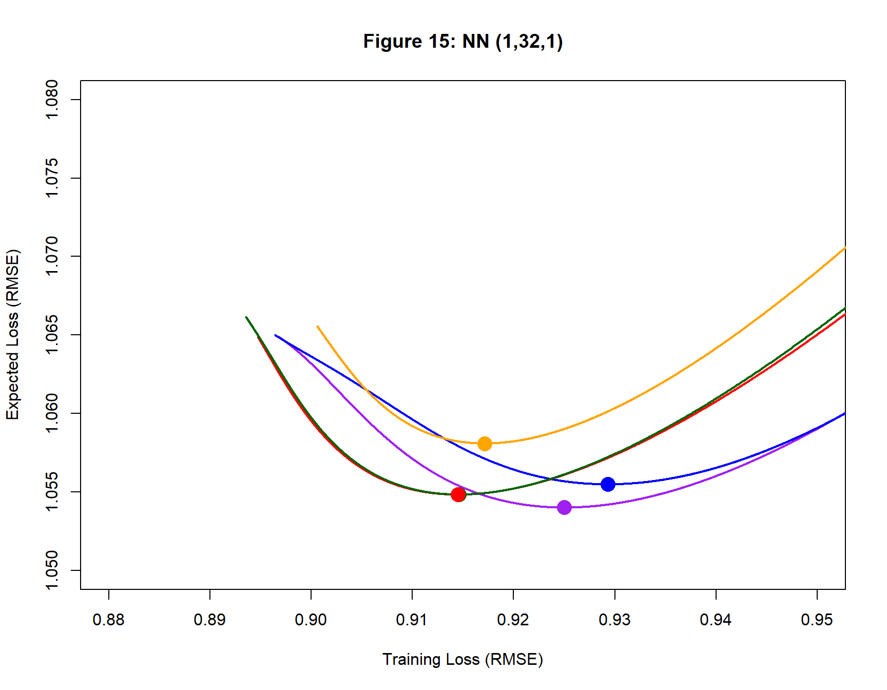
Analysis 4: A (1, 32, 1) Neural Network
Next, the data are analysed using a (1, 32, 1) neural network. This model has 97 parameters, far more that are needed for the simple Gausaain curve. I use a step length of 0.05 to avoid oscillation. The results are shown in figure 15 and table 5.
The green and red paths almost overlap and the weights and biases of their fitted models are similar. The performance of this over-parameterised model is remarkably similar to that of the 13 parameter model used in the first analysis.
| Table 5: Neural Network (1, 32, 1) eta=0.05 | |||||||
| Details of the Fitted Model | |||||||
| Colour | Iteration | Loss (RMSE) | Weights | Biases | |||
|---|---|---|---|---|---|---|---|
| Training | Expected | mean | std | mean | std | ||
| Purple | 3930 | 0.925 | 1.054 | 0.26 | 3.52 | 0.08 | 3.45 |
| Blue | 4009 | 0.929 | 1.055 | −0.53 | 3.86 | 0.16 | 3.23 |
| Red | 6058 | 0.914 | 1.055 | −1.06 | 3.50 | 0.08 | 3.28 |
| Dark Green | 4612 | 0.915 | 1.055 | −0.65 | 3.82 | 1.29 | 3.19 |
| Orange | 6761 | 0.917 | 1.058 | 0.00 | 3.77 | 0.55 | 3.39 |
| Average | 5074 | 0.920 | 1.055 | −0.40 | 3.70 | 0.43 | 3.31 |
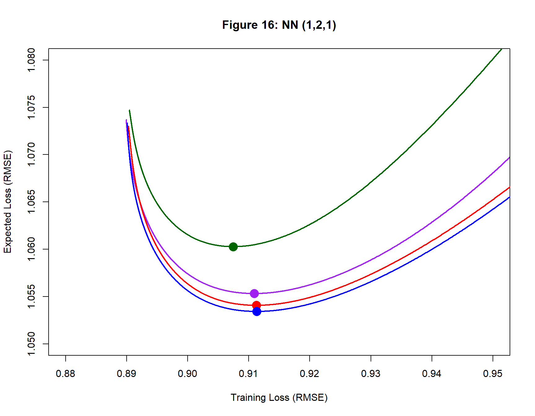
Analysis 5: A (1, 2, 1) Neural Network
Finally, the data are analysed using a model with only 7 parameters; a (1, 2, 1) neural network that is probably a little under-parameterised for a Gaussian curve. For this analysis, I revert to a step length of 0.1. The results are shown in figure 16 and table 6.
Figure 16 only shows four search paths because the fifth (orange) did not have any training or expected RMSE below 1.65.
| Table 5: Neural Network (1, 2, 1) | |||||||
| Details of the Fitted Models | |||||||
| Colour | Iteration | Loss (RMSE) | Weights | Biases | |||
|---|---|---|---|---|---|---|---|
| Training | Expected | mean | std | mean | std | ||
| Purple | 4069 | 0.911 | 1.055 | 5.31 | 9.87 | −3.71 | 3.48 |
| Blue | 1931 | 0.911 | 1.053 | −4.70 | 9.95 | 2.30 | 8.04 |
| Red | 2609 | 0.911 | 1.054 | −4.48 | 10.12 | 2.17 | 8.28 |
| Dark Green | 4982 | 0.907 | 1.060 | 5.78 | 9.90 | −2.96 | 7.45 |
| Orange | 10000 | 1.690 | 1.660 | 3.45 | 7.26 | −2.97 | 2.68 |
| Average | 4718 | 1.066 | 1.177 | 1.07 | 9.42 | −1.03 | 5.99 |
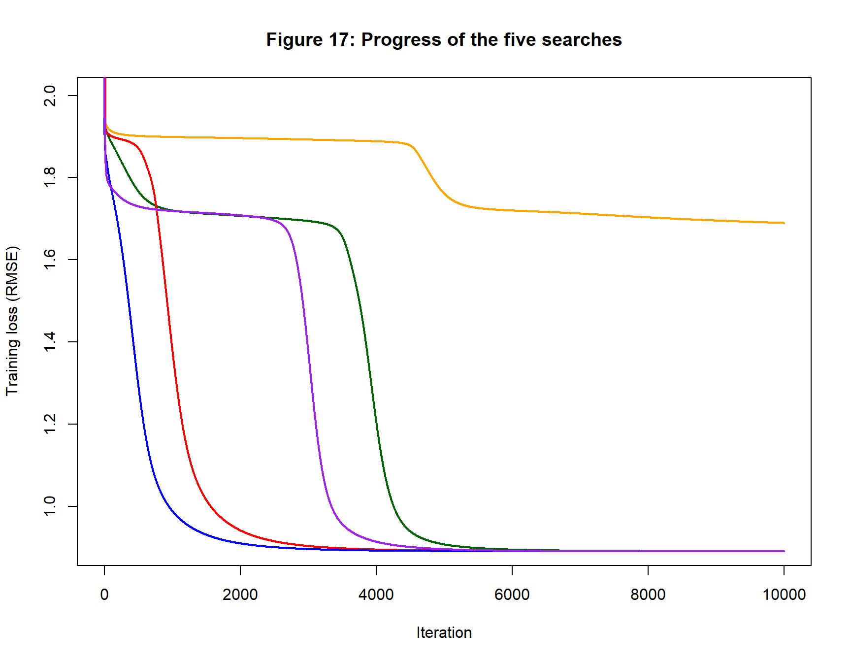
The progress of training loss of the five searches is shown in figure 17. The shape of the unsuccessful search is not dissimilar to the others except that it does not drop as far. Just like the others, it consists of periods of rapid loss reduction followed by long plateaus. It is unclear whether the orange curve would dip again were the algorithm run for long enough, or whether it has converged to a local minimum that is a long way from the Best model.
Comparing these Models
Table 6 collects together the averages from the tables of fitted model statistics. It is remarkable how neural networks of different size produce models with such similar training and expected loss.
| Table 6: Average performance | |||||||||
| Details of the Fitted Models | |||||||||
| Model | eta | p1 | Iteration | Loss (RMSE) | Weights | Biases | |||
|---|---|---|---|---|---|---|---|---|---|
| Training | Expected | mean | std | mean | std | ||||
| 1, 2, 1 | 0.10 | 7 | 4718 | 1.066 | 1.177 | 1.07 | 9.42 | −1.03 | 5.99 |
| 1, 4, 1 | 0.10 | 13 | 2102 | 0.911 | 1.055 | 1.02 | 7.45 | −0.84 | 4.13 |
| 1, 8, 1 | 0.10 | 25 | 1892 | 0.914 | 1.054 | 0.27 | 5.54 | 0.55 | 4.03 |
| 1, 16, 1 | 0.10 | 49 | 2887 | 0.917 | 1.056 | 0.33 | 4.60 | −0.18 | 3.83 |
| 1, 16, 1 | 0.05 | 49 | 5322 | 0.919 | 1.056 | 0.40 | 4.58 | 0.22 | 3.68 |
| 1, 32, 1 | 0.05 | 97 | 5074 | 0.920 | 1.055 | −0.40 | 3.70 | 0.43 | 3.31 |
| 1 p = Number of parameters | |||||||||
Conclusions
Flexible regression is a particularly simple use of neural networks, none the less, it highlights many of the features of gradient descent. In the next post, I will consider ways of simulating multi-dimensional data for analysis by larger neural networks, meanwhile here are some of the important messages from this post.
- Neural networks with very different looking parameters can have the same expected loss and/or the same training loss.
- Unless the training set is very large, a low training loss does not imply a low expected loss, so the training loss is a poor indicator of future performance.
- Running gradient descent until the training loss converges to a minimum is not a good strategy.
- When a model is selected based on having a low training loss, that final loss will exaggerate the performance of the model on future data.
- Model selection should be based on the loss in a large dataset that is independent of the training data. Such datasets rarely exist in practice.
- It is impossible to tell from a single run of gradient descent whether or not the algorithm is close to the best model, so always run gradient descent from a range of starting values.
- Oscillation or increasing training loss indicate that a smaller step size should be used.
- Over-parameterised neural networks perform remarkably well. The main disadvantage of having too many parameters is the increased computation time.
- It is better to use a neural network with too many parameters than one with too few.
Losses calculated by resampling are often used as a practical alternative to the expected loss. I will write a separate post on cross-validated and bootstrap losses and investigate whether they are good substitutes for the expected loss.
Appendix: Code Changes
I added a function cfit_valid_nn() that is a modification of cfit_nn(). It runs gradient descent in exactly the same way, but allows the user to specify {XV, YV}, a holdout sample used to estimate the expected loss. The new function trains using the training data exactly as before, but also returns the iteration by iteration validation loss.
The new code also changes the way that the activation functions are specified to give the potential for a different activation function for each layer.
C code with these changes can be found on my GitHub pages as cnnUpdate01.cpp.