Neural Networks: C Code for Gradient Descent
Introduction
In my previous post, I described my R Code for fitting a neural network (NN) by gradient descent. Those R functions are computationally intensive and as R is a notoriously slow language, the R code is only useful for fitting relatively small networks and would be impractical for studying the performance of NNs on multiple simulated datasets. Before starting my investigations of NNs, this R code needs to be rewritten in a faster language and in common with most R users, I have chosen to use C.
The R package, Rcpp, allows C or C++ code to be seamlessly integrated into R and is widely used to speed up the internal workings of R packages. The computations needed to fit a NNs are relatively simple and as a result the C code needed will itself be very straightforward; little more than loops and basic arithmetic operations.
Needless to say, this conversion from R to C will make little sense unless you have first read my previous post on R functions for fitting NNs.
The C language
C is a relatively old language that has been updated many times. It is a compiled language in which every variable has a defined type, such as integer or character or float. The combination of compilation and strict typing produces code that is extremely quick. Despite its age, C is still one of the fastest computer languages.
Here are a few features of C to keep in mind when reading my code.
- lines of C code end in a semi-colon
- C uses = for assignment where R uses <-
- comments start with // where R uses #
- blocks of C code are enclosed in curly brackets { } just as in R
- arrays in C are indexed starting at zero, while R starts indexing at one
- basic C does not have complex data structures built-in such as R’s matrix or list
- in C, every object has a type that must be specified before the object is used. In contrast, R has dynamic typing and is not strict at all
Of these features the one that is most problematic for R users is the indexing that starts at 0. Even though you know it, it is so easy to forget.
The Rcpp package
The Rcpp package does two jobs, first it compiles C and C++ code and integrates it into R in such a way that the user is unaware whether computation is being performed by C or R. Second, it provides C equivalents to many of R’s complex structures. In this way, an R matrix or an R list can be passed directly to a function written in C and that C function can return its results in a structure that R will recognise and use.
The Conversion
Let’s dive in. I will explain the details of C and Rcpp as they arise.
The C functions that I write have been placed in a file called cnnOriginal.cpp, a copy of which can be found on my GitHub pages.
prepare_nn() to cprepare_nn()
The first of my R functions is called prepare_nn(), it creates the data structures and pointers used by the fitting algorithm. The main change is that whereas my R example had 8 nodes numbered 1 to 8, in C they are numbered 0 to 7. I call the adapted version cprepare_nn().
The code for cpreprare_nn() is given below. Here are some things to notice
archdescribes the architecture of the network, e.g. (4, 5, 1) means 3 layers with 4 input nodes, a single hidden layer of 5 nodes and an output layer with 1 node.
IntegerVectoris a type defined by Rcpp, it denotes a vector of integers
IntegerVector (10)defines a vector of exactly 10 integers
x.length()returns the length of the vector x
x += 5is shorthand forx = x + 5
x++is shorthand for adding 1 to x
intis the standard C type for a single integer
for(int i=0; i<5; i++) {...}creates a loop equivalent to R’sfor(i in 0:4) {...}
Rcpp::runif()is a function supplied by Rcpp for generating random numbers. The equivalent base R function can be obtained usingR::runif()
- The cumbersome code for creating a named
List(capital L) is part of Rcpp
cpreprare_nn()takes a single vector of integers as its input and returns aList
// function to return pointers and initial values for an arbitrary NN
// inputs
//    arch  the architecture of the network
// output
//    a List of pointers and initial values
//
List cprepare_nn(IntegerVector arch) {
  // Number of layers
  int nLayers = arch.length();
  // Number of Nodes
  int nNodes = 0;
  for(int j = 0; j < nLayers; j++) nNodes += arch[j];
  // Pointer to first Node of each layer
  IntegerVector nPtr (nLayers+1);
  int h = 0;
  for(int j = 0; j < nLayers; j++) {
    nPtr[j] = h;
    h += arch[j];
  }
  nPtr[nLayers] = nNodes;
  // number of weights for a fully connected NN
  int nWt = 0;
  for(int j = 1; j < nLayers; j++) nWt += arch[j-1] * arch[j];
  // origin and destination of each node
  IntegerVector from (nWt);
  IntegerVector to (nWt);
  int q1 = 0;
  int q2 = 0;
  h = 0;
  for(int j = 1; j < nLayers; j++) {
    q1 += arch[j-1];
    for(int f = 0; f < arch[j-1]; f++ ) {
      for(int t = 0; t < arch[j]; t++ ) {
        from[h] = f + q2;
        to[h] = t + q1;
        h++;
      }
    }
    q2 = q1;
  }
  // Pointer to the first weight of each layer
  IntegerVector wPtr (nLayers);
  for(int j = 1; j < nLayers - 1; j++) {
     wPtr[j] = wPtr[j-1] + arch[j-1] * arch[j];
  }
  wPtr[nLayers - 1] = nWt;
  // Random Starting Values
  NumericVector bias = Rcpp::runif(nNodes, -1.0, 1.0);
  NumericVector weight = Rcpp::runif(nWt, -1.0, 1.0);
  // return the design
  List L = List::create(Named("bias") = bias ,
                        _["weight"]   = weight,
                        _["from"]     = from,
                        _["to"]       = to,
                        _["nPtr"]     = nPtr,
                        _["wPtr"]     = wPtr);
  return L;
}
As an illustration, here are the C pointers for a 3 layer NN with 2 inputs, 3 hidden nodes and 1 output.
design <- cprepare_nn( c(2, 3, 1))
str(design)
## List of 6
## $ bias : num [1:6] 0.5324 0.0835 0.326 0.2829 0.4449 ...
## $ weight: num [1:9] 0.016 0.779 0.797 -0.278 0.601 ...
## $ from : int [1:9] 0 0 0 1 1 1 2 3 4
## $ to : int [1:9] 2 3 4 2 3 4 5 5 5
## $ nPtr : int [1:4] 0 2 5 6
## $ wPtr : int [1:3] 0 6 9forward_nn() to cforward_nn()
The R function forward_nn() makes a forward pass through the network calculating the value of each node. The R version was given in my previous post, it takes the design created by prepare_nn() as one of its inputs and assumes that functions for the activation functions have been defined by the user.
Below is the C version. I decided to pass the components of the design rather than the list, but I could have passed the list and unpacked it inside of cforward_nn(); an arbitrary decision on my part.
// function to make a forward pass through a NN
// inputs
//    v the values of each node (input nodes must be set before calling this function)
//    bias the bias of each node
//    weight the weights of the network
//    from the source of each weight (from cprepare_nn)
//    to the destination of each weight (from cprepare_nn)
//    nPtr pointer to first node of each layer (from cprepare_nn)
//    wPtr pointer to first weight of each layer (from cprepare_nn)
// output
//    v the updated values of each node
// requires
//    cActHidden() activation function to be applied to hidden nodes
//    cActOutput() activation to be applied to output nodes
//
NumericVector cforward_nn(NumericVector v,
                          NumericVector bias,
                          NumericVector weight,
                          IntegerVector from,
                          IntegerVector to,
                          IntegerVector nPtr,
                          IntegerVector wPtr) {
  // Size of network
  int nLayers = nPtr.length() - 1;
  int nNodes  = v.length();
  // z = linear combinations inputs to each node
  // v = value of each node v = activation(z)
  NumericVector z(nNodes);
  for(int i = 0; i < nNodes; i++) {
    z[i] = bias[i];
  }
  for(int i = 1; i < nLayers; i++) {
    for(int k = nPtr[i]; k < nPtr[i+1]; k++ ) {
      for(int h = wPtr[i-1]; h < wPtr[i]; h++) {
        if( to[h] == k ) {
          z[k] += weight[h] * v[from[h]];
        }
      }
      // apply activation function
      if( i < nLayers - 1 )
        v[k] = cActHidden( z[k]);
      else
        v[k] = cActOutput( z[k]);
    }
  }
  return v;
}
The C code is pretty self-explanatory. It allows different activation functions to be applied to the hidden and output nodes. cActHidden() and cActOutput() must be supplied separately by the user.
backprop_nn() to cbackprop_nn()
Next comes the back-propagation function cbackprop_nn(). The original is in my previous post. Notice the way that the results are packed into a named List.
// function to make a backward pass through a NN calculating the derivatives of the
// weights and biases corresponding to a single observation yi
// inputs
//    y the single observation
//    v the current values of each node
//    bias the bias of each node
//    weight the weights of the network
//    from the source of each weight (from cprepare_nn)
//    to the destination of each weight (from cprepare_nn)
//    nPtr pointer to first node of each layer (from cprepare_nn)
//    wPtr pointer to first weight of each layer (from cprepare_nn)
// output
//    List containing the derivatives of the loss wrt the weights and biases
// requires
//    cdActHidden() derivative of activation function to be applied to hidden nodes
//    cdActOutput() derivative of activation to be applied to output nodes
//    cdloss() derivative of the loss
//
List cbackprop_nn(NumericVector y,
                  NumericVector v,
                  NumericVector bias,
                  NumericVector weight,
                  IntegerVector from,
                  IntegerVector to,
                  IntegerVector nPtr,
                  IntegerVector wPtr) {

  // Size of network
  int nLayers = nPtr.length() - 1;
  int nNodes  = bias.length();
  int nWts    = weight.length();
  int nY      = y.length();
  // define structures
  double wjk  = 0.0;
  NumericVector dbias(nNodes);
  NumericVector dweight(nWts);
  NumericVector dv(nNodes);
  NumericVector df(nNodes);
  NumericVector yhat(nY);
  NumericVector dLoss(nY);
  // df = derivatives of activation functions
  // yhat = predicted network outputs
  for(int j = nPtr[1]; j < nPtr[nLayers-1]; j++) {
    df[j] = cdActHidden(v[j]);
  }
  for(int j = nPtr[nLayers-1]; j < nPtr[nLayers]; j++) {
    df[j] = cdActOutput(v[j]);
    yhat[j-nPtr[nLayers-1]] = v[j];
  }
  // derivative of loss wrt to yhat
  dLoss = cdLoss(y, yhat);
  // dv derivatives of loss wrt each nodal value
  // dbias derivatives of loss wrt the bias
  // dweight derivatives of loss wrt the weights
  for(int j = nPtr[nLayers-1]; j < nPtr[nLayers]; j++) {
    dv[j] = dLoss[j-nPtr[nLayers-1]];
  }
  for(int i = nLayers-1; i > 0; i-- ) {
    for(int j = nPtr[i]; j < nPtr[i+1]; j++) {
      dbias[j] = dv[j] * df[j];
      for(int h = wPtr[i-1]; h < wPtr[i]; h++) {
        if( to[h] == j) {
          dweight[h] = dv[j] * df[j] * v[from[h]];
        }
      }
    }
    for(int j = nPtr[i-1]; j < nPtr[i]; j++) {
      dv[j] = 0.0;
      for(int k = nPtr[i]; k < nPtr[i+1]; k++) {
        for(int h = wPtr[i-1]; h < wPtr[i]; h++) {
          if( (from[h] == j) & (to[h] == k) ) wjk = weight[h];
        }
        dv[j] += dv[k] * df[k] * wjk;
      }
    }
  }
  // return derivatives as a named list
  List L = List::create(Named("dbias") = dbias ,
                        _["dweight"] = dweight);
  return L;
}
fit_nn() to cfit_nn()
Next is the function fit_nn() that iterates over the training data. This function is called directly by the user from within R so I decided to simplify the arguments by passing the design as a List, which I unpack inside the function.
// fits a neural network by gradient descent
// inputs
//    X matrix of training data (predictors)
//    Y matrix of training data (responses)
//    design list as returned by cpreprare_nn()
//    eta the learning rate (step length)
//    nIter number of iterations of the algorithm
//    trace whether to report progress 1=yes 0=no
// returns list of results containing
//    bias the biases of the final model
//    weight the weights of the final model
//    lossHistory the loss after each iteration
//    dbias derivatives of loss wrt the bias after the final iteration
//    dweight derivative of loss wrt the weights after the final iteration
//  requires
//    closs() calculates the loss function
//
List cfit_nn( NumericMatrix X,
              NumericMatrix Y,
              List design,
              double eta = 0.1,
              int nIter  = 1000,
              int trace  = 1 ) {
  // unpack the design
  IntegerVector from   = design["from"];
  IntegerVector to     = design["to"];
  IntegerVector nPtr   = design["nPtr"];
  IntegerVector wPtr   = design["wPtr"];
  NumericVector bias   = design["bias"];
  NumericVector weight = design["weight"];
  // size of the training data
  int nr = X.nrow();
  int nX = X.ncol();
  int nY = Y.ncol();
  // problem size and working variables
  int nNodes   = bias.length();
  int nWts     = weight.length();
  double tloss = 0.0;
  NumericVector v (nNodes);
  NumericVector yhat (nY);
  NumericVector y (nY);
  NumericVector lossHistory (nIter);
  NumericVector dw (nWts);
  NumericVector db (nNodes);
  // iterate nIter times
  for( int iter = 0; iter < nIter; iter++ ) {
    // set derivatives & loss to zero
    for(int i = 0; i < nWts;   i++) dw[i] = 0.0;
    for(int i = 0; i < nNodes; i++) db[i] = 0.0;
    tloss = 0.0;
    // iterate over the rows of the training data
    for( int d = 0; d < nr; d++) {
      // set the predictors into v
      for(int i = 0; i < nX; i++) v[i] = X(d, i);
      // forward pass
      v = cforward_nn(v, bias, weight, from, to, nPtr, wPtr);
      // extract the predictions
      for(int i = 0; i < nY; i++) {
        yhat[i] = v[nNodes - nY + i];
        y[i]    = Y(d, i);
      }
      // calculate the loss
      tloss += closs(y, yhat);
      // back-propagate and unpack
      List deriv = cbackprop_nn(y, v, bias, weight, from, to, nPtr, wPtr);
      NumericVector dweight = deriv["dweight"];
      NumericVector dbias   = deriv["dbias"];
      // sum the derivatives
      for(int i = 0; i < nWts;   i++) dw[i] += dweight[i];
      for(int i = 0; i < nNodes; i++) db[i] += dbias[i];
    }
    // save loss and update the parameters
    lossHistory[iter] = tloss / nr;
    for(int i = 0; i < nWts; i++) weight[i] -= eta * dw[i] / nr;
    for(int i = 0; i < nNodes; i++) bias[i] -= eta * db[i] / nr;
    // report loss every 100 iterations
    if( (trace == 1) & (iter % 100 == 0) ) {
      Rprintf("%i %f \n", iter, tloss / nr);
    }
  }
  // return the results
  List L = List::create(Named("bias")    = bias ,
                        _["weight"]      = weight,
                        _["lossHistory"] = lossHistory,
                        _["dbias"]       = db / nr,
                        _["dweight"]     = dw / nr);
  return L;
}
Notice the use of Rprintf() to write output to the console
predict_nn() to cpredict_nn()
predict_nn() is a convenience R function that makes predictions for a set of predictors saved in a matrix X. It makes repeated calls to forward_nn(). The C equivalent is called cpredict_nn() and the code is self-explanatory.
// predictions for a fitted NN
// inputs
//    X matrix of test data (predictors)
//    design list as returned by cpreprare_nn()
// returns
//    Y a matrix of predictions
//
NumericMatrix cpredict_nn( NumericMatrix X,
                           List design) {
  // unpack the design
  IntegerVector from   = design["from"];
  IntegerVector to     = design["to"];
  IntegerVector nPtr   = design["nPtr"];
  IntegerVector wPtr   = design["wPtr"];
  NumericVector bias   = design["bias"];
  NumericVector weight = design["weight"];
  // size of the test data
  int nr = X.nrow();
  int nX = X.ncol();
  int nLayers = nPtr.length() - 1;
  int nNodes = bias.length();
  int nY = nPtr[nLayers] - nPtr[nLayers-1];
  NumericVector a (nNodes);
  NumericMatrix Y (nr, nY);
  // iterate over the rows of the test data
  for( int d = 0; d < nr; d++) {
    // set the predictors into a
    for(int i = 0; i < nX; i++) a[i] = X(d, i);
    // forward pass
    a = cforward_nn(a, bias, weight, from, to, nPtr, wPtr);
    // extract the predictions
    for(int i = 0; i < nY; i++) Y(d, i) = a[nNodes - nY + i];
  }
  // return the predictions
  return Y;
}
Problem specific functions
The functions that calculate the loss, the activation functions and their derivatives are problem specific, but here is the code for a squared error loss and a sigmoid activation function.
// Problem specific C functions

double closs(NumericVector y, NumericVector yhat) {
  double loss = 0.0;
  int nY = y.length();
  for(int i = 0; i < nY; i++) loss += (y[i] - yhat[i])*(y[i] - yhat[i]);
  return loss;
}

NumericVector cdLoss(NumericVector y, NumericVector yhat) {
  return -2.0 * (y - yhat);
}

double cActHidden(double z) {
  return 1.0 / (1.0 + exp(-z));
}

double cActOutput(double z) {
      return z;
    }

double cdActHidden(double a) {
      return a * (1.0 - a);
    }

double cdActOutput(double a) {
      return 1.0;
    }
The cnnOriginal.cpp file
All of the above C code needs to be place in a single .cpp file. Mine is called cnnOriginal.cpp. The file must start
#include <Rcpp.h>
using namespace Rcpp;
and any functions that you want to call directly from R, as opposed to C functions called by other C functions, must be exported. This is achieved by preceding them by the comment.
// [[Rcpp::export]]Now the .cpp file can be compiled using standard R code
library(Rcpp)

# Source the C functions
sourceCpp("C:/Projects/Sliced/methods/methods_neural_nets/C/cnnOriginal.cpp")
The Quadratic Example
Now to test the code. I use exactly the same dataset that I used for the R equivalent functions in my previous post.
library(Rcpp)

# Source the C functions
sourceCpp("C:/Projects/Sliced/methods/methods_neural_nets/C/cnnOriginal.cpp")

# Simulate and plot some training data
set.seed(7109)
X <- matrix(runif(15, 0, 1), nrow = 15, ncol = 1)
Y <- matrix(3*(X[,1]-0.5)^2 + rnorm(15, 0, 0.2), nrow = 15, ncol = 1)
plot(X[, 1], Y[, 1], pch = 16, main = "The training data")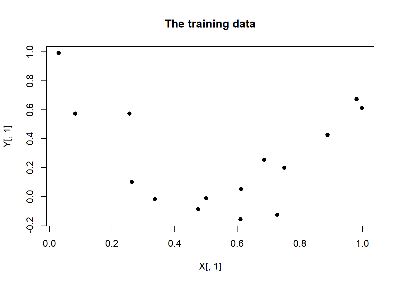
# create the network design
set.seed(8923)
arch  <- c(1, 4, 1)
design <- cprepare_nn(arch)
str(design)
## List of 6
## $ bias : num [1:6] 0.47234 0.00661 -0.42113 0.00113 -0.10775 ...
## $ weight: num [1:8] 0.1419 -0.675 -0.5684 0.71 0.0493 ...
## $ from : int [1:8] 0 0 0 0 1 2 3 4
## $ to : int [1:8] 1 2 3 4 5 5 5 5
## $ nPtr : int [1:4] 0 1 5 6
## $ wPtr : int [1:3] 0 4 8# Fit the model
start_time <- Sys.time()
fit <- cfit_nn(X, Y, design, eta=0.1, nIter = 10000, trace=0)
end_time <- Sys.time()
print(end_time - start_time)## Time difference of 0.2708299 secs# plot the history of the loss
plot(fit$lossHistory, type = "l", ylim = c(0, 0.2))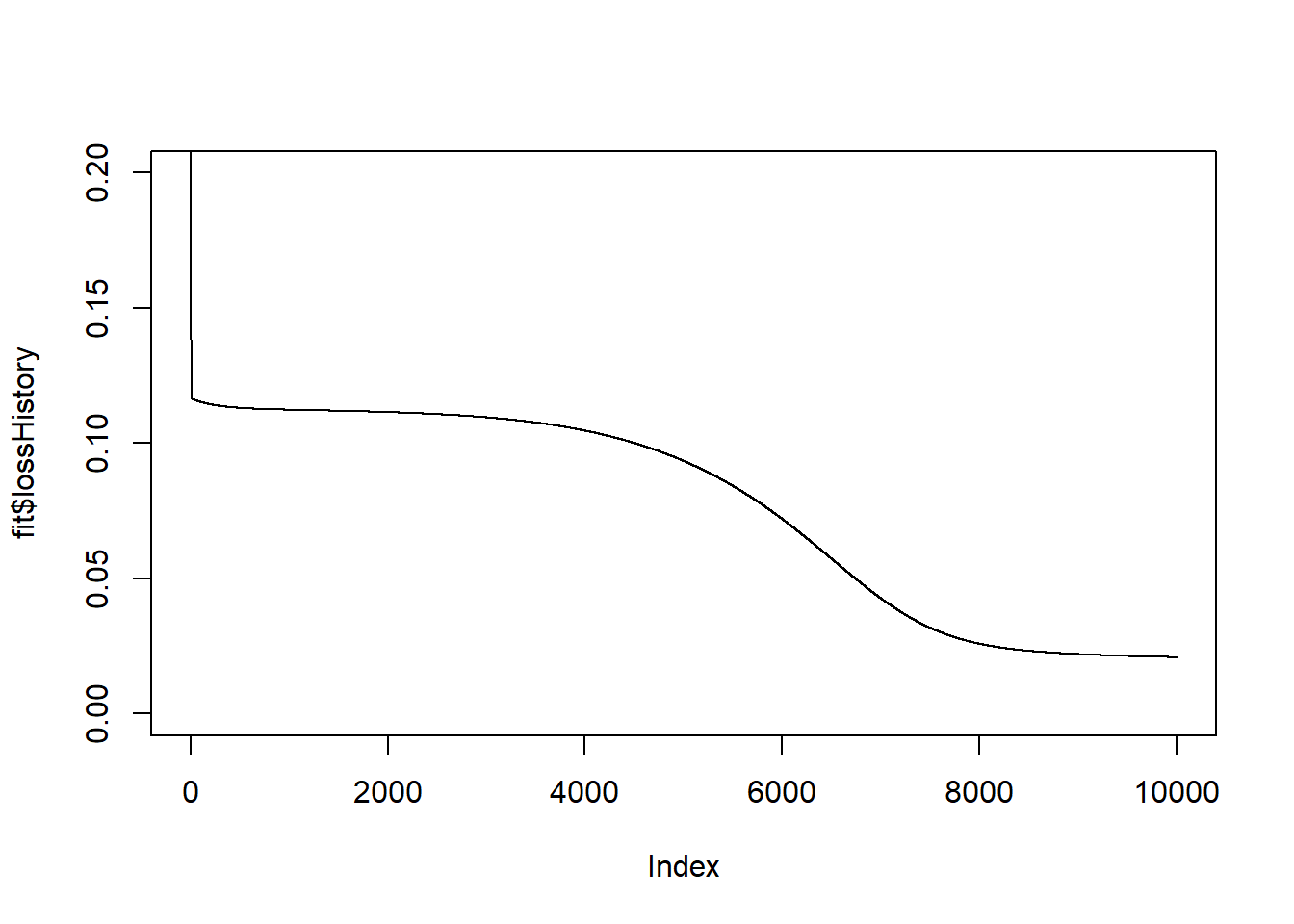
# Look at the fit
design$bias   <- fit$bias
design$weight <- fit$weight
# selected values of x for the plot
xt <- matrix(seq(0, 1, 0.02), ncol=1)
# make prediction for each xt
yt <- cpredict_nn(xt, design)

# plot the predictions against the inputs over the training data
plot(X[, 1], Y[, 1], pch = 16, main = "NN model after 10000 iterations")
lines(xt[, 1], yt[, 1])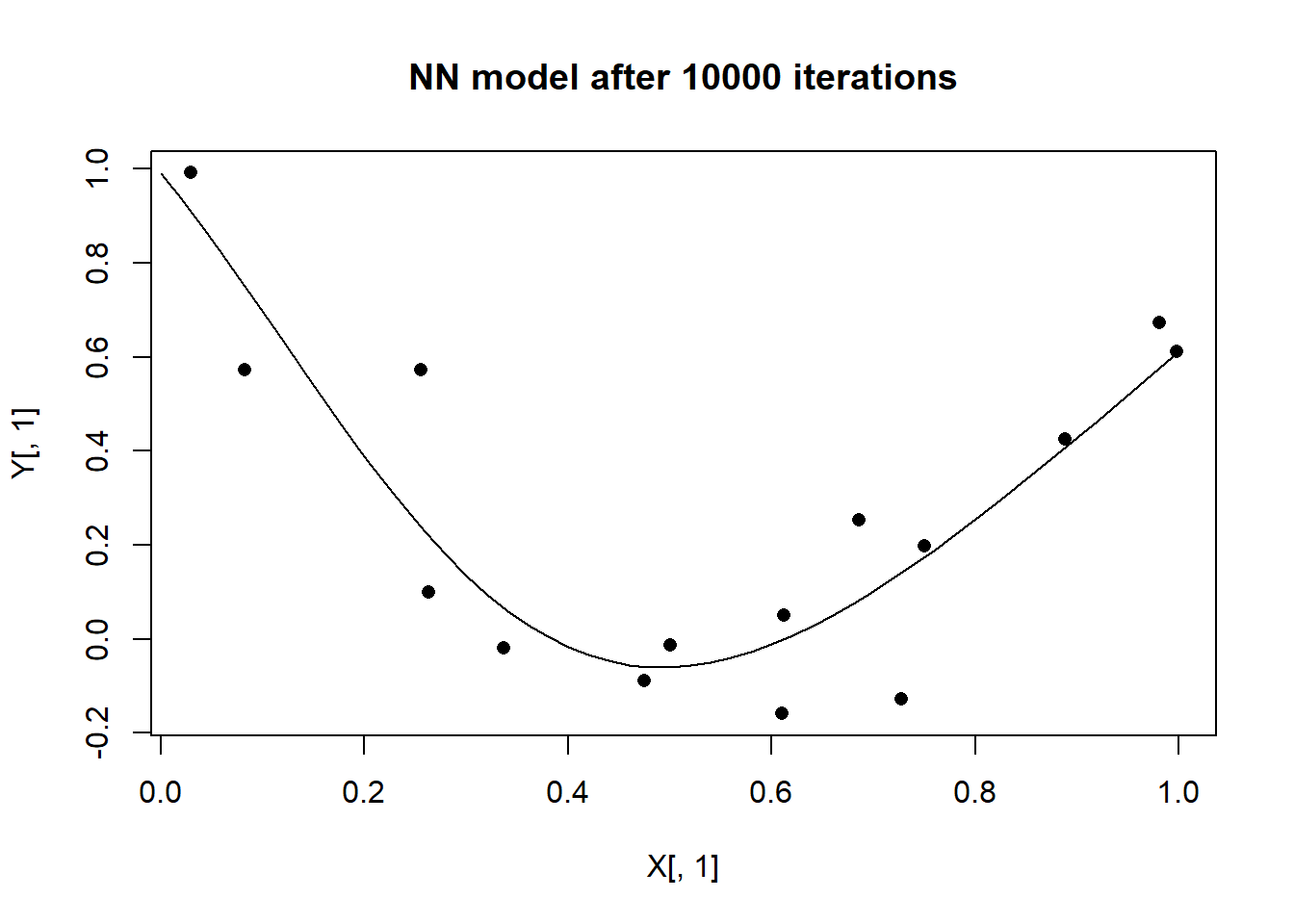
The results are equivalent to those obtained with R code accept that C runs 12 times quicker.
The time saving increases with the number of parameters in the model. A (1,4,1) NN has 13 parameters and runs 12 times faster in C. A (1, 4, 4, 1) NN has 31 parameters and runs 48 times faster in C.
Conclusions
The C code is much, much quicker, even though the gain is not that great in the simple quadratic example.