Creating predictions

First a recap; in my introductory post on NNs, I used the example of a NN with 8 nodes arranged in 4 layers and explained that I like to number the nodes in order, in this case 1 to 8, and to give each node a value denoted \(v_1\) to \(v_8\).

The first two nodes make up the input layer and are set equal to the values of the predictors, x1 and x2, \[ v_1 = x_{1} \ \ \ \ \text{and} \ \ \ v_2 = x_{2} \]

The calculation for each subsequent node can be split into two stages. Using \(v_3\) as an example, the first stage calculates \(z_3\) as a simple linear combination of the inputs,
\[ z_3 = \beta_3 + \beta_{13} v_1 + \beta_{23} v_2 \] The second stage converts \(z_3\) into \(v_3\) using the activation function, f().
\[ v_3 = f(z_3) \]

In my R code, I place the values of z, v and the biases in vectors of length 8, even though the first two elements of v have known values and the corresponding elements of z and the biases will never be used.

Because the calculations are performed, layer by layer, it is convenient to have a pointer that tells where within these vectors each layer begins and ends. In this case, the pointer is (1, 3, 6, 8), meaning that layer 2 starts with node 3 and finishes with node 5 (6-1).

There are 14 weights represented by arrows in the diagram. These weights are placed in a vector in the order (13, 14, 15, 23, 24, 25, 36, 37, 46, 47, 56, 57, 68, 78), where 37 means the weight connecting node 3 to node 7. A second pointer that identifies the layer of origin of each arrow, In this case, it is (1, 7, 13)

Eventually, the R code will need to create these design variables from a description of the network’s architecture, but for the moment I will manually create values specific to this example and also generate random weights and biases.

# first node of each layer
nPtr <- c(1, 3, 6, 8, 9)
# starting and finishing node for each weight
from <- c(1, 1, 1, 2, 2, 2, 3, 3, 4, 4, 5, 5, 6, 7)
to   <- c(3, 4, 5, 3, 4, 5, 6, 7, 6, 7, 6, 7, 8, 8)
# first weight of each layer
wPtr <- c(1, 7, 13, 15)
# Space for v and z
v <- rep(0, 8)
z <- rep(0, 8)
# Random values for the bias and weight
set.seed(5561)
bias <- runif(8, -1, 1)
weight <- runif(14, -1, 1)

For coding convenience my pointers include a extra value that is one more than the length of the corresponding vector.

I apply a sigmoid activation function to the hidden nodes, this will convert z to an activated value, v, that lies between 0 and 1. The plot below shows the shape of this activation function.

z <- seq(-4, 4, 0.1)
v <- 1 /( 1 + exp(-z))
plot(z, v, type = "l", main = "Sigmoid Activation Function")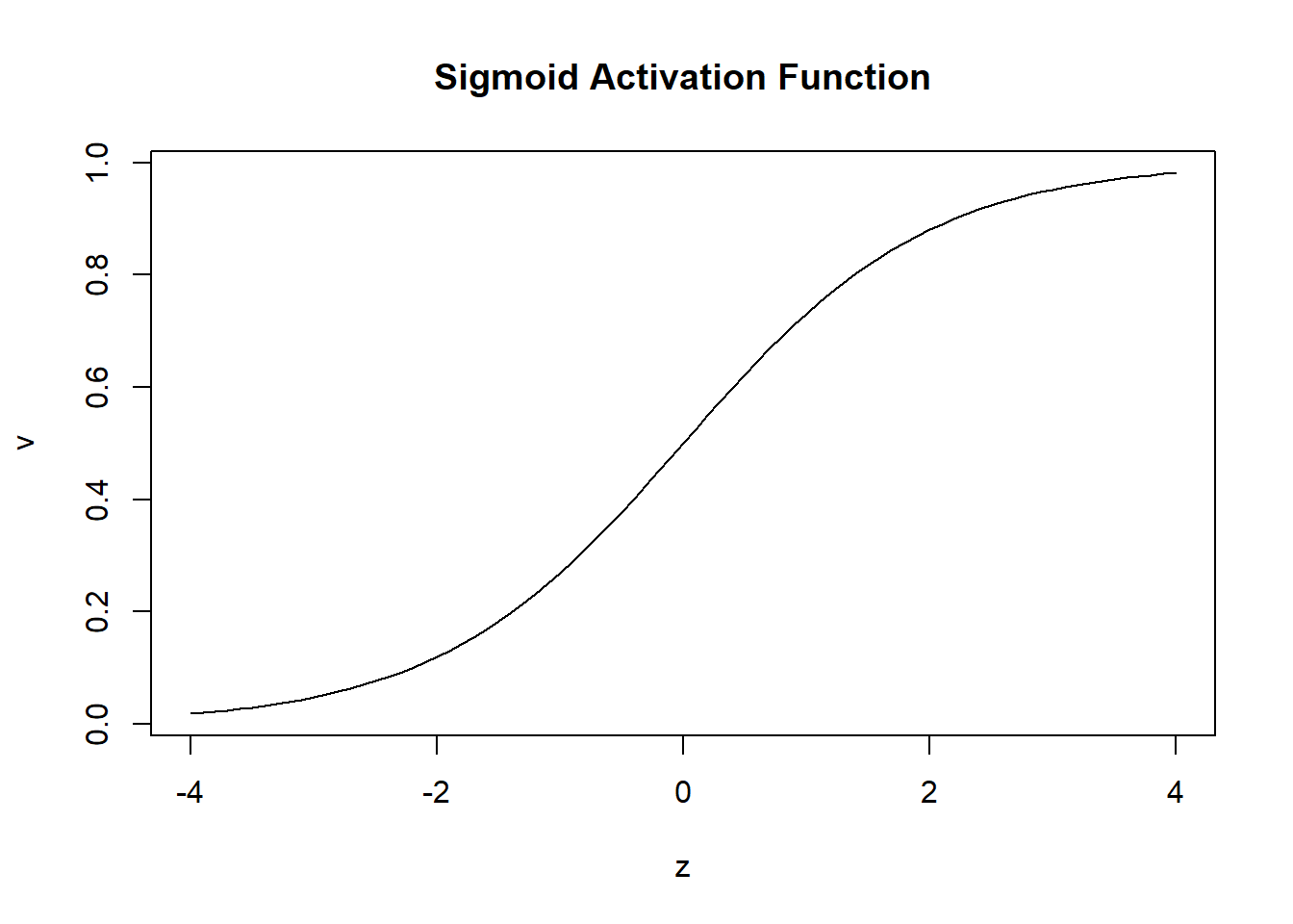

The sigmoid is a popular choice, but many others have been suggested.

Since, in my regression example, y is unbounded, I will not apply any activation to the final prediction but instead set \(v_8 = z_8\).

Suppose that the first observation in the training data is (x1 = 3.1, x2 = 2.7, y = 0.3). The following code calculates the value v of each node. v includes the predicted value of y, which is found in the output layer.

The weights and biases have been set randomly, so we should not expect the prediction from this NN to be accurate.

# set the values of the input layer
v    <- rep(0, 8)
v[1] <- 3.1
v[2] <- 2.7
# set z equal to the bias
z <- bias
# for layers 2 to 4
for(i in 2:4) {
  # for each node in this layer
  for(j in nPtr[i]:(nPtr[i+1]-1)) {
    # weights that originate in the previous layer
    for(h in wPtr[i-1]:(wPtr[i]-1)) {
      # does the weight go to node j?
      if( to[h] == j ) {
        # add (weight * value) to z
        z[j] <- z[j] + weight[h] * v[from[h]]
      }
    }
    # apply the sigmoid activation function to hidden nodes
    if( i != 4 ) {
      v[j] <- 1.0 / (1.0 + exp(-z[j]))
    } else {
      v[j] <- z[j]
    }
  }
}
print(v)

## [1]  3.10000000  2.70000000  0.07676566  0.56151852  0.98352402  0.74555848
## [7]  0.68832585 -0.59856899

As expected, these random weights produce a poor prediction, \(v_8\), of -0.5986, when y is actually 0.3.

For illustration, I use the usual mean square loss \[ L(y, \mu) = \frac{1}{n} \sum_{i = 1}^n (y_i - \mu_i)^2 \]

So for the single training observation the loss is 0.807.

y <- 0.3
loss <- (y - v[8])^2
print(loss)

## [1] 0.8074262

Gradient Descent

Random parameters give poor estimates and a high loss, but they act as starting values for an algorithm that progressively reduces the loss.

In order to select appropriate adjustments to the weights and biases, I calculate the derivative of the loss with respect to each of the 20 parameters (weights + biases). Then I use these derivatives to guide a small adjustment in a downhill direction. There are no guarantees that changing all of the parameters at once in this way will reduce the loss, but it is a reasonable strategy that works most of the time, especially when the step sizes of the adjustments are kept small.

Computing the 20 derivatives in a way that is generalisable is easier that it might at first seem, provided that we work backwards through the network. The algorithm that calculates the derivatives in this way is known as back-propagation.

In terms of the v’s the loss function is \[ L(y, \mu) = \frac{1}{n} \sum_{i = 1}^n (y_i - v_{8i})^2 \] For simplicity, I’ll drop the i suffix that refers to the ith observation in the training data. In practice, the algorithm cycles through each training observation in turn and sums the results, so all we really need is R code that works for a single training observation. The simplified loss is, \[ L(y, \mu) = (y - v_8)^2 \] and the derivative of the loss with respect to \(v_8\) is \[ \frac{\partial L}{\partial v_8} = -2 (y - v_8) \]

Since no activation function is applied at the final stage, \(z_8 = v_8\) and \[ \frac{\partial L}{\partial z_8} = \frac{\partial L}{\partial v_8} \]

The diagram of the network shows that \[ z_8 = \beta_8 + \beta_{68} v_6 + \beta_{78} v_7 \] where \(v_6\) and \(v_7\) have already been calculated as part of the forward step that found the prediction, \(v_8\).

The derivative of the loss with respect to the bias, \(\beta_8\), is \[ \frac{\partial L}{\partial \beta_8} = \frac{\partial L}{\partial z_8} \frac{\partial z_8}{\partial \beta_8} = -2 (y - v_8) \ \ \text{x} \ \ 1 \] and the derivative of the loss with respect to the weight, \(\beta_{68}\), is \[ \frac{\partial L}{\partial \beta_{68}} = \frac{\partial L}{\partial z_8} \frac{\partial z_8}{\partial \beta_{68}} = -2 (y - v_8) \ \ \text{x} \ \ v_6 \] A similar formula gives the derivative with respect to \(\beta_{78}\), \[ \frac{\partial L}{\partial \beta_{78}} = \frac{\partial L}{\partial z_8} \frac{\partial z_8}{\partial \beta_{78}} = -2 (y - v_8) \ \ \text{x} \ \ v_7 \]

We can also calculate the derivative with respect to \(v_6\). Although this is not of direct interest, it is needed when the next layer of derivatives is calculated. \[ \frac{\partial L}{\partial v_6} = \frac{\partial L}{\partial z_8} \frac{\partial z_8}{\partial v_6} = -2 (y - v_8) \ \ \text{x} \ \ \beta_{68} \] where \(\beta_{68}\) is the current value of that weight.

Moving backwards through the NN from layer 4 to layer 3, \[ z_6 = \beta_6 + \beta_{36} v_3 + \beta_{46} v_4 + \beta_{56} v_5 \] A sigmoid activation function is used in this layer, so I need to include the derivative of \(v_6\) with respect to \(z_6\). Since \(v_6 = f(z_6)\), this is just the derivative of the activation function. In the case of the sigmoid, this derivative is \(v_6(1-v_6)\)

Putting this all together, the derivative with respect to the bias, \(\beta_6\), is, \[ \frac{\partial L}{\partial \beta_6} = \frac{\partial L}{\partial v_6} \frac{\partial v_6}{\partial z_6} \frac{\partial z_6}{\partial \beta_6} \] I calculated the partial with respect to \(v_6\) in the previous layer and the partial of \(z_6\) with respect to \(\beta_6\) is one.

This pattern continues as we move backwards through the network. It is very repetitive, so, with care, it can be coded.

In my code, I create three vectors of length 8 to hold the derivatives of the loss with respect to (wrt) the bias and wrt v and the derivative of the activation function. A vector of length 14 holds the derivatives of the loss wrt the weights.

# vectors for the derivatives
dbias <- dv <- df <- rep(0, 8)
dweight <- rep(0, 14)
# the training response
y <- 0.3
# derivatives of the activation functions
for(j in 3:7) {
  df[j] <- v[j]*(1-v[j])
}
df[8] <- 1
# final layer dloss/da
dv[8] <- -2 * (y - v[8])
# move backwards through the layers
for(i in 4:2) {
  # for each node in that layer
  for( j in nPtr[i]:(nPtr[i+1]-1) ) {
     # dloss/dbias
     dbias[j] <- dv[j] * df[j] * 1
     # dloss/dweight
     # for weights that end at node j
     for( h in wPtr[i-1]:(wPtr[i]-1) ) {
        if( to[h] == j ) {
           dweight[h] <- dv[j] * df[j] * v[from[h]]
        }
     }
  }
  # dloss/dv - may involve multiple routes
  for( j in nPtr[i-1]:(nPtr[i]-1) ) {
     dv[j] <- 0
     for( k in nPtr[i]:(nPtr[i+1]-1) ) {
        for(h in wPtr[i-1]:(wPtr[i]-1) ) {
           if( from[h] == j & to[h] == k) wjk <- weight[h]
        }
        dv[j] <- dv[j] + dv[k] * df[k] * wjk
     }
  }
}
print(dbias)

## [1]  0.0000000000  0.0000000000 -0.0020395917 -0.0088170206  0.0001177478
## [6] -0.0347579283 -0.1432396942 -1.7971379872

print(dweight)

##  [1] -0.0063227343 -0.0273327637  0.0003650183 -0.0055068976 -0.0238059555
##  [6]  0.0003179192 -0.0026682155 -0.0109958903 -0.0195172206 -0.0804317416
## [11] -0.0341852575 -0.1408796803 -1.3398714709 -1.2370165354

These derivatives tell us the direction to move in. To reduce the loss we must move against the gradient. I’ll make my step length, eta, equal to 0.1. In machine learning eta is usually called the learning rate.

# step length
eta <- 0.1
# steps down hill
weight <- weight - eta * dweight
bias   <- bias   - eta * dbias

With these adjusted parameters we can recalculate the prediction and the loss

# repeat the forward pass to create a new prediction
z <- bias
for(i in 2:4) {
  for(j in nPtr[i]:(nPtr[i+1]-1)) {
    for(h in wPtr[i-1]:(wPtr[i]-1)) {
      if( to[h] == j ) {
        z[j] <- z[j] + weight[h] * v[from[h]]
      }
    }
    if( i != 4 ) {
      v[j] <- 1.0 / (1.0 + exp(-z[j]))
    } else {
      v[j] <- z[j]
    }
  }
}
print(v[8])

## [1] -0.229929

loss <- (y - v[8])^2
print(loss)

## [1] 0.2808248

The loss has been reduced from 0.807 to 0.281. Now we just repeat and repeat.

NN Fitting Functions

In the R code below, I have generalized this fitting process so that it works with any neural network architecture. The user must specify the number of nodes in each layer, the loss function, the activation function and their derivatives.

The function prepare_nn() will generate random starting values together with pointers to the start of each layer and it also creates the to and from vectors that link the weights to the nodes.

# Takes the architecture arch and creates pointers and random starting values
# arch = c(2, 3, 2, 1) means 4 layers with 2 predictors and 1 response 
prepare_nn <- function(arch) {
  nLayers <- length(arch)
  nNodes  <- sum(arch)
  nPtr <- rep(0, nLayers+1)
  # pointer to the first node in a layer
  h <- 1
  for( j in 1:nLayers) {
    nPtr[j] <- h
    h <- h + arch[j]
  }
  nPtr[nLayers+1] <- nNodes+1
  # number of weights
  nWt <- 0
  for( j in 2:nLayers) {
    nWt <- nWt + arch[j-1] * arch[j]
  }
  # node origin and destination of each weight
  from <- to <- rep(0, nWt)
  q1 <- q2 <- h <- 0
  for( i in 2:nLayers) {
    q1 <- q1 + arch[i-1]
    for(f in 1:arch[i-1]) {
      for(t in 1:arch[i]) {
        h <- h + 1
        from[h] <- f + q2
        to[h]   <- t + q1
      }
    }
    q2 <- q1
  }
  # pointer to the first weight in each layer
  wPtr<- rep(0, nLayers)
  for( h in 1:nWt) {
    for( i in 1:(nLayers-1)) {
      if( from[h] == nPtr[i] & wPtr[i] == 0 ) {
        wPtr[i] <- h  
      }
    }
  }
  wPtr[nLayers] <- nWt + 1
  # random starting values
  bias <- runif(nNodes, -1, 1)
  weight <- runif(nWt, -1, 1)
  # return the design
  return( list(bias = bias, weight = weight, 
               from = from, to = to, 
               nPtr = nPtr, wPtr = wPtr))
}

To test the code, I run this function for the demonstration network and get the same design as I entered manually earlier in this post.

set.seed(5561)
design <- prepare_nn( c(2, 3, 2, 1))
str(design)

## List of 6
##  $ bias  : num [1:8] -0.7712 0.2912 -0.3997 0.4239 -0.0587 ...
##  $ weight: num [1:14] -0.423 0.688 0.502 -0.288 -0.855 ...
##  $ from  : num [1:14] 1 1 1 2 2 2 3 3 4 4 ...
##  $ to    : num [1:14] 3 4 5 3 4 5 6 7 6 7 ...
##  $ nPtr  : num [1:5] 1 3 6 8 9
##  $ wPtr  : num [1:4] 1 7 13 15

The forward pass through the network that calculates the value for each node is coded in the function forward_nn(). The user needs to provide the activation function for the nodes in the hidden layers and a separate activation function for the nodes in the output layer.

# The activation functions
actHidden <- function(z) {
  return(1.0 / (1.0 + exp(-z)))
}
actOutput <- function(z) {
  return(z)
}

The values of the vector v can now be calculated.

# Move forward through the network calculating each node's value, v
# inputs (predictors) must be entered into v before calling this function
forward_nn <- function(v, design) {
  nLayers <- length(design$nPtr) - 1
  # set z equal to the bias
  z <- design$bias
  # for layers 2 onwards
  for(i in 2:nLayers) {
    # for each node in this layer
    for(j in design$nPtr[i]:(design$nPtr[i+1]-1)) {
      # weights that originate from layer i-1
      for(h in design$wPtr[i-1]:(design$wPtr[i]-1)) {
        # does the weight go to node j?
        if( design$to[h] == j ) {
          # add (weight * value) to z
          z[j] <- z[j] + design$weight[h] * v[design$from[h]]
        }
      }
      # apply the sigmoid activation function to hidden nodes
      if( i != nLayers ) {
        v[j] <- actHidden(z[j])
      } else {
        v[j] <- actOutput(z[j])
      }
    }
  }
  return(v)
}

Once again, I use the demonstration NN as a test

v <- rep(0, length(design$bias))
v[1] <- 3.1
v[2] <- 2.7
v <- forward_nn(v, design)
print(v)

## [1]  3.10000000  2.70000000  0.07676566  0.56151852  0.98352402  0.74555848
## [7]  0.68832585 -0.59856899

Reassuringly, I get the same prediction as before, \(v_8\) = -0.5986.

Next, I need a function for back-propagation. At this stage, the user must specify their loss and the derivatives of that loss and the derivatives of the activation functions.

# loss function
loss <- function(y, yhat) {
  return( (y-yhat)^2 )
}
# derivative of loss wrt prediction
dLoss <- function(y, yhat) {
  return( -2*(y-yhat))
}
# derivative of hidden layer activation
dActHidden <- function(v) {
  return(v*(1-v))
}
# derivative of output layer activation
dActOutput <- function(v) {
  return(1)
}

With these functions defined, back-propagation is performed by the function backprop_nn().

# back-propagate the derivatives
backprop_nn <- function(y, v, design) {
  nLayers <- length(design$nPtr) - 1
  nNodes  <- length(v)
  nWts    <- length(design$weight)    
  dbias   <- dv <- df <- rep(0, nNodes)
  dweight <- rep(0, nWts)
  nX      <- design$nPtr[2] - design$nPtr[1]
  nY      <- length(y)
  yhat    <- rep(0, nY)
  # derivatives of the activation functions
  for(j in nPtr[2]:(nNodes-nY) ) {
    df[j] <- dActHidden(v[j])
  }
  for(j in (nNodes-nY+1):nNodes ) {
    df[j] <- dActOutput(v[j])
    yhat[j-nNodes+nY] <- v[j]
  }
  # final layer dloss/dv
  dv[nNodes] <- dLoss(y, yhat)
  # move backwards through the layers
  for(i in nLayers:2) {
    # for each node in that layer
    for( j in design$nPtr[i]:(design$nPtr[i+1]-1) ) {
      # dloss/dbias
       dbias[j] <- dv[j] * df[j]
       # dloss/dweight
       # for weight that ends at node j
       for( h in design$wPtr[i-1]:(design$wPtr[i]-1) ) {
         if( design$to[h] == j ) {
           dweight[h] <- dv[j] * df[j] * v[design$from[h]]
         }
       }
    }
    # dloss/dv - may involve multiple routes
    for( j in design$nPtr[i-1]:(design$nPtr[i]-1) ) {
      dv[j] <- 0
      for( k in design$nPtr[i]:(design$nPtr[i+1]-1) ) {
        for(h in design$wPtr[i-1]:(design$wPtr[i]-1) ) {
           if( design$from[h] == j & design$to[h] == k) 
             wjk <- design$weight[h]
        }
        dv[j] <- dv[j] + dv[k] * df[k] * wjk
      }
    }
  }
  return(list(dbias = dbias, dweight = dweight))
}

For the demonstration example the derivatives of the parameters are,

deriv <- backprop_nn(0.3, v, design)
str(deriv)

## List of 2
##  $ dbias  : num [1:8] 0 0 -0.00204 -0.008817 0.000118 ...
##  $ dweight: num [1:14] -0.006323 -0.027333 0.000365 -0.005507 -0.023806 ...

Using these derivatives to adjust the parameters improves the loss exactly as it did when I used my problem specific code.

# old loss
ls <- loss(0.3, v[8])
print(ls)

## [1] 0.8074262

# adjust the parameters
eta <- 0.1
design$bias   <- design$bias   - eta * deriv$dbias
design$weight <- design$weight - eta * deriv$dweight
# new prediction
v <- forward_nn(v, design)
print(v)

## [1]  3.10000000  2.70000000  0.07702481  0.56540056  0.98352061  0.74663794
## [7]  0.69565422 -0.22992901

# new loss
ls <- loss(0.3, v[8])
print(ls)

## [1] 0.2808248

My next function, fit_nn(), takes a set of training data saved in matrices X and Y and iterates the forward pass and back-propagation.

# fit a NN to training data (X, Y)
fit_nn <- function(X, Y, design, eta = 0.1, nIter = 1000, trace=TRUE ) {
  # size of the training data
  nr <- nrow(X)
  nX <- ncol(X)
  nY <- ncol(Y)
  # problem size and working variables
  nNodes  <- length(design$bias)
  nWts    <- length(design$weight)    
  v <- rep(0, nNodes)
  yhat <- rep(0, nY)
  lossHistory <- rep(0, nIter)
  # iterate nIter times
  for( iter in 1:nIter) {
    # set derivatives & loss to zero
    dw <- rep(0, nWts)
    db <- rep(0, nNodes)
    tloss <- 0
    # iterate over the rows of the training data
    for( d in 1:nr ) {
       # set the predictors into a
       for(i in 1:nX) {
         v[i] <- X[d, i]
       }
       # forward pass
       v <- forward_nn(v, design)
       # extract the predictions
       for(i in 1:nY) {
         yhat[i] <- v[nNodes-nY+i]
       }
       # calculate the loss 
       tloss <- tloss + loss(as.numeric(Y[d, ]), yhat)
       # backpropagate
       deriv <- backprop_nn(as.numeric(Y[d, ]), v, design)
       # sum the derivatives
       dw <- dw + deriv$dweight
       db <- db + deriv$dbias
    }
    # save loss and update the parameters
    lossHistory[iter] <- tloss / nr
    design$weight <- design$weight - eta * dw / nr
    design$bias   <- design$bias   - eta * db / nr
    # print loss
    if( trace & iter %% 100 == 0) {
      cat(iter, " ", tloss/nr, "\n")
    }
  }
  # return the results
  return(list(bias = design$bias, weight = design$weight, 
              lossHistory = lossHistory,
              dbias = db/nr, dweight = dw/nr))
}

Finally, there is a function to calculate the predictions for a test set of data X.

predict_nn <- function(X, design) {
  # size of the training data
  nr <- nrow(X)
  nX <- ncol(X)
  nLayers <- length(design$nPtr) - 1;
  nNodes <- length(design$bias);
  nY <- design$nPtr[nLayers+1] - design$nPtr[nLayers];
  Y <- matrix(0, nrow=nr, ncol=nY)
  v <- rep(0, nNodes)
  for( d in 1:nr ) {
    # set the predictors into a
    for(i in 1:nX) {
      v[i] <- X[d, i]
    }
    # forward pass
    v <- forward_nn(v, design)
    # extract the predictions
    for(i in 1:nY) {
      Y[d, i] <- v[nNodes-nY+i]
    }
  }
  return(Y)
}

Let’s test this code with some simulated data. For ease of display, I have chosen a problem with a single predictor and a single output. The training set has 15 observations generated from a quadratic with a small amount of random error.

# Simulate some training data
set.seed(7109)
X <- matrix(runif(15, 0, 1), nrow = 15, ncol = 1)
Y <- matrix(3*(X[,1]-0.5)^2 + rnorm(15, 0, 0.2), nrow = 15, ncol = 1)
plot(X[, 1], Y[, 1], pch = 16, main = "The training data")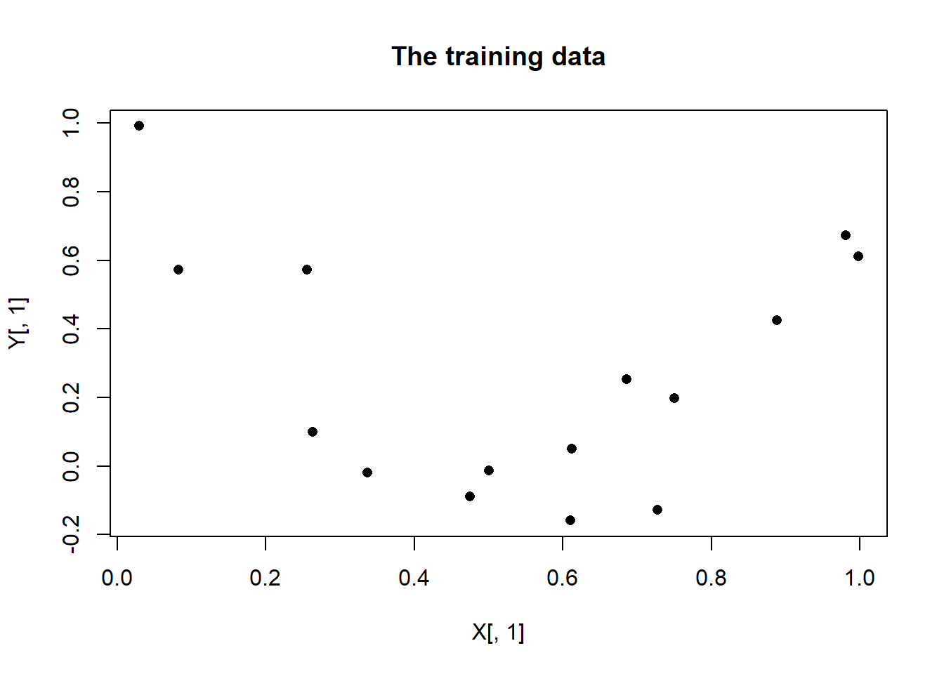

I’ll model these data with a NN that has a single hidden layer containing 4 nodes.

# create the network design
set.seed(8923)
design <- prepare_nn(c(1, 4, 1))
str(design)

## List of 6
##  $ bias  : num [1:6] 0.47234 0.00661 -0.42113 0.00113 -0.10775 ...
##  $ weight: num [1:8] 0.1419 -0.675 -0.5684 0.71 0.0493 ...
##  $ from  : num [1:8] 1 1 1 1 2 3 4 5
##  $ to    : num [1:8] 2 3 4 5 6 6 6 6
##  $ nPtr  : num [1:4] 1 2 6 7
##  $ wPtr  : num [1:3] 1 5 9

When I run 1000 iterations, the loss is reduced a little. There is a big improvement in the loss in the first few iterations, but little change after that.

fit <- fit_nn(X, Y, design, eta=0.1, nIter = 1000)

## 100   0.1153072 
## 200   0.1144552 
## 300   0.1138409 
## 400   0.1133947 
## 500   0.1130678 
## 600   0.1128253 
## 700   0.1126414 
## 800   0.1124976 
## 900   0.1123801 
## 1000   0.1122794

plot(fit$lossHistory, type = "l", ylim = c(0, 0.2))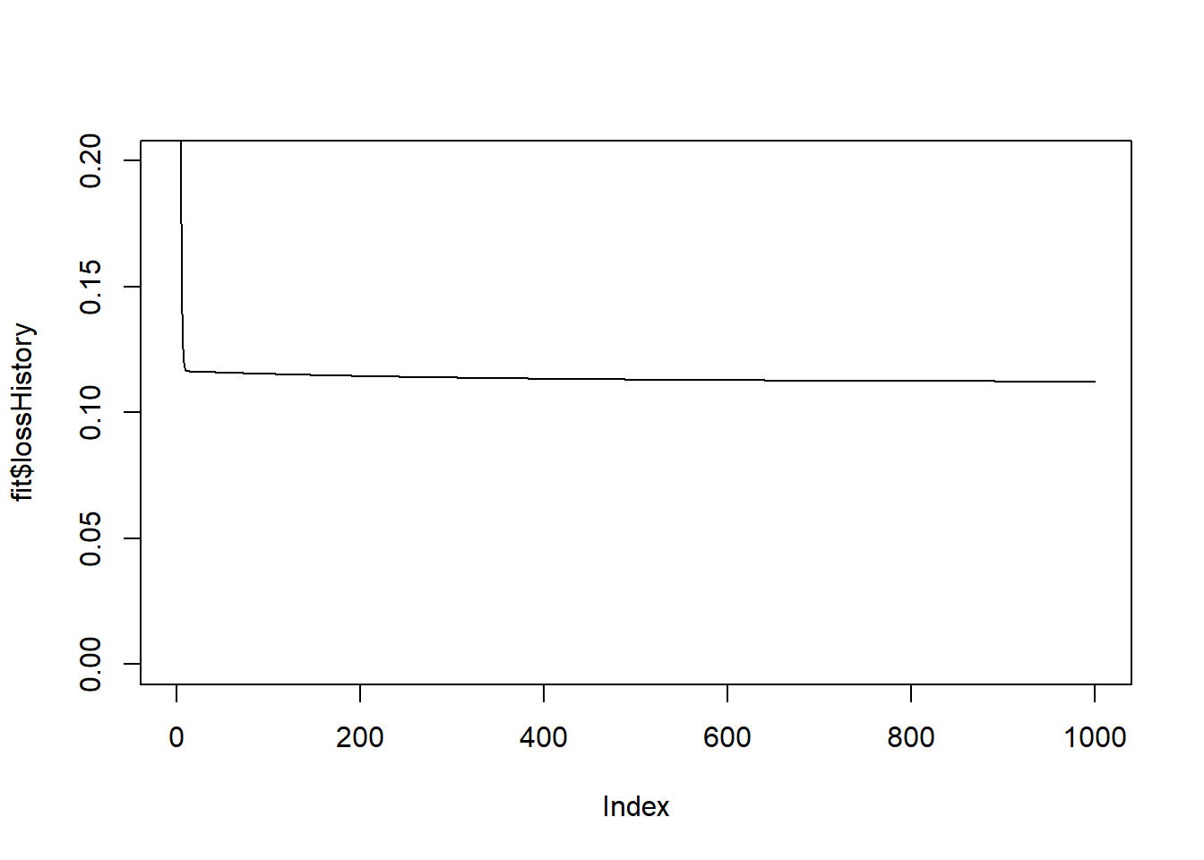

We can visualise the model suggested by this NN by making predictions at a sequence of values between 0 and 1.

design$bias   <- fit$bias
design$weight <- fit$weight
# selected values of x
xt <- matrix(seq(0, 1, 0.02), ncol=1)
# make prediction for each xt
yt <- predict_nn(xt, design)
# plot the predictions
plot(X[, 1], Y[, 1], pch = 16, main = "NN model after 1000 iterations")
lines(xt[, 1], yt[, 1])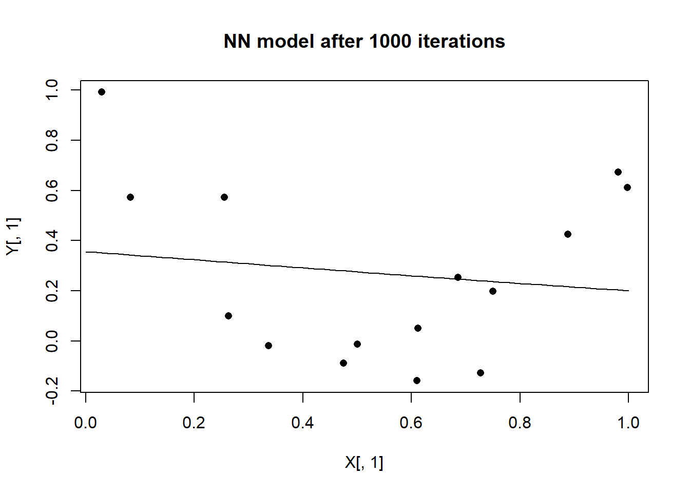

The network has fitted a straightish line through the points. Hopefully, this will be improved upon when I run more iterations.

start_time <- Sys.time()
fit <- fit_nn(X, Y, design, eta=0.1, nIter = 10000, trace=FALSE)
end_time <- Sys.time()
print(end_time - start_time)

## Time difference of 3.992728 secs

plot(fit$lossHistory, type = "l", ylim = c(0, 0.2))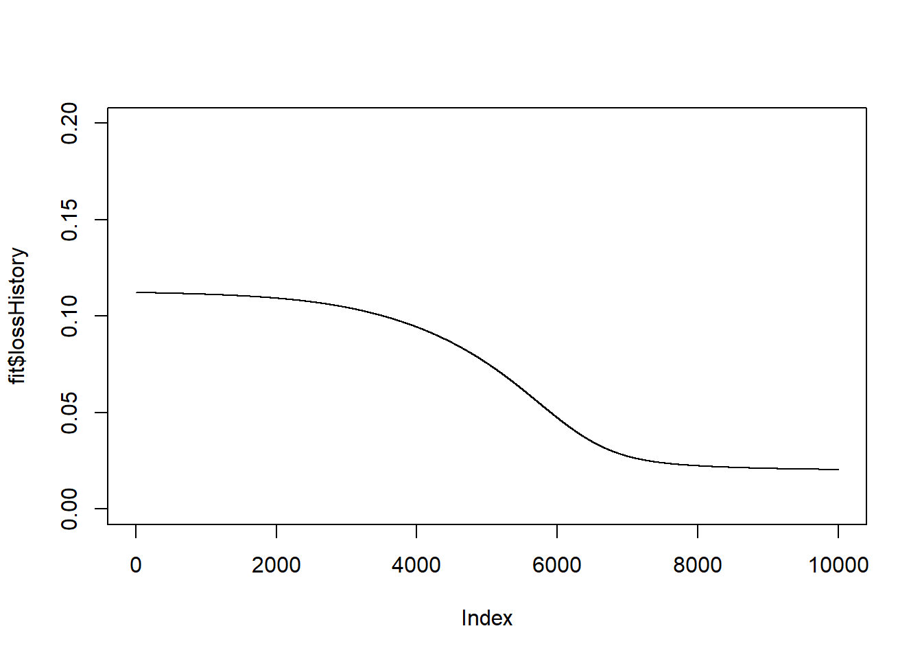

It only takes a few seconds for the algorithm to locate a better solution.

Plotting the predictions from this latest model shows that the NN has discovered a better approximation to the shape of the response curve.

design$bias   <- fit$bias
design$weight <- fit$weight
# make prediction for each xt
yt <- predict_nn(xt, design)

# plot the predictions
plot(X[, 1], Y[, 1], pch = 16, main = "NN model after 11000 iterations")
lines(xt[, 1], yt[, 1])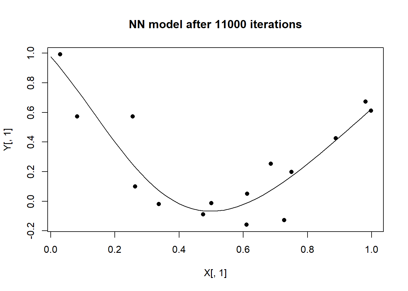

Conclusions

Even this simple example raises many questions.

• why a (1, 4, 1) architecture?
  
• how would I tell that 1000 iterations was not enough if it were not possible to plot the data, say because there were multiple x’s or multiple y’s?
  
• what would happen if I ran 100,000 iterations?
• why a step size (learning date) of 0.1? Would other step sizes work better?
  
• could the step size be adjusted as the algorithm progresses?
  
• would alternative activation functions produce a better model?
  
• how critical are the random starting values?
  
• do all starting values lead to the same final NN?
  
• are there different sets of parameters that produce more or less the same loss?
  
• is the successful performance, specific to this particular random set of 15 observations?
  
• would the NN still find the quadratic if the data had a larger random component?
  
• could a small change in the training data cause the NN to choose a very different response curve?
  
• would convergence be improved if I scaled the training data?
  
• are there any clues in the data that would help me choose the architecture of the network?

I do what to investigate these and other questions, but first I will speed up the computation by converting my R code to C++. That will be the topic for my next post.